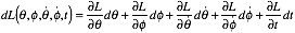
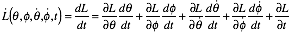
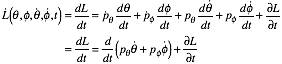
Unit 2 Lagrangian and Hamiltonian Mechanics
W. G. Harter
Methods of Lagrange and Hamilton are used to solve problems in generalized curvilinear coordinates. Practical aspects of these methods are shown by constructing and analyzing equations of motion including those of an ancient war machine called the trebuchet or ingenium. Also treated are pendulum oscillation and electromagnetic cyclotron dynamics that are used to introduce phase space and analytic and computational power of Hamiltonian theory. Some analogies of trebuchet mechanics with sports biomechanics provide a lesson on how you might improve your tennis or golf swing!
Trebuchet forces and equations of motion
___________________________________________________________________________________
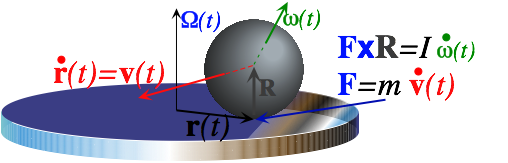
Mechanical analog for cyclotron dynamics
Unit 2. Lagrangian and Hamiltonian Mechanics........................................... 5
Chapter 1. The Trebuchet: A dream problem for Galileo?.............................................................................................. 5
Chapter 2. Generalized Curvilinear Coordinates (GCC) and derivatives........................................................................... 11
Relating GCC to CC (Cartesian coordinates)..................................................................................................... 11
Generalized coordinate differentials....................................................................................................................... 11
Jacobians.................................................................................................................................................... 14
Kajobians................................................................................................................................................... 15
Generalized velocity.......................................................................................................................................... 17
Lemma 1:  (2.2.14)................................................................................................................ 17
Generalized acceleration..................................................................................................................................... 17
Lemma 2:  (2.2.16)................................................................................................................ 18
Chapter 3. Lagrangian GCC derivatives and kinetic energy........................................................................................... 19
Lagrangian derivative equations....................................................................................................................... 20
Kinetic energy in GCC: Metric Tensors γμν........................................................................................................... 20
Understanding and checking Lagrangian expressions............................................................................................ 20
Understanding the dynamic metric γμν............................................................................................................... 21
Arm inertia............................................................................................................................................. 22
Chapter 4. Canonical momentum in Lagrange equations: dp/dt=F.................................................................................. 23
How Lagrange equations hide fictitious and constraint forces.................................................................................... 24
Chapter 5. Riemann equations of motion.................................................................................................................. 27
Checking torques and acceleration.................................................................................................................... 27
Trebuchet model force inventory..................................................................................................................... 28
Chapter 6. Lagrangian and Hamiltonian equations of motion....................................................................................... 31
Do we define force like mathematician (F= +ÑV) or physicist (F= -ÑV)?............................................................... 31
Hamiltonian equations of motion........................................................................................................................ 32
Legendre-Poincare relation H=p•v-L................................................................................................................. 32
L is function of v while H is a function of p..................................................................................................... 33
Hamilton’s vs. Lagrange’s equations................................................................................................................ 33
What good are Hamilton's equations?................................................................................................................... 34
Conservation laws........................................................................................................................................ 34
Symmetry and conservation (No lumps? No bumps!).......................................................................................... 34
Conjugate variables...................................................................................................................................... 34
Lagrange-Poincare invariant action.................................................................................................................. 35
Momentum symmetry means no-go................................................................................................................ 35
Chapter 7. Hamiltonian mechanics of pendulum oscillation......................................................................................... 37
Hamiltonian phase space................................................................................................................................... 39
Small-amplitude motion: the "eye" of a storm....................................................................................................... 41
Other benefits of Hamiltonians: The Liouville theorem....................................................................................... 43
Other benefits of Hamiltonians : Virial relations................................................................................................ 44
Power-law Hamiltonians............................................................................................................................... 44
Approximate quantum E-levels................................................................................................................... 44
Chapter 8. Charged particle in electromagnetic fields................................................................................................... 47
Levi-Civita again......................................................................................................................................... 47
Hamiltonian for charged particle in fields.............................................................................................................. 48
Cyclotron orbits in E and B fields....................................................................................................................... 49
Hall-effect drift............................................................................................................................................ 49
The FBI right-hand rule................................................................................................................................. 51
Mechanical analogy for cyclotron motion in magnetic field.................................................................................. 53
Chapter 9. Idealization, analogy, and analysis of trebuchet motion................................................................................. 57
Trebuchet-sports analogies: Aristotle vs Newton and flinger vs trebuchet.................................................................... 57
Semi-quantitative comparison: trebuchet vs. flinger............................................................................................ 59
Experiments for comparing trebuchet vs. flinger................................................................................................ 62
Linear and parametric resonance: Trebuchets and twiddling................................................................................... 64
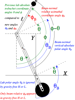
Hamiltonian gravity-free trebuchet kinematics....................................................................................................... 66
Coordinate kinetics in gravity-free (g=0) case..................................................................................................... 66
Advanced trebuchet mechanics............................................................................................................................ 70
References.......................................................................................................................................................... 73
Unit 1 Review Topics and Formulas........................................................................................................................ 74
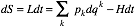
BANG! A fiendish 30-ton war machine hurls a 5-ton load of rocks, garbage, and bodies of plague victims onto panicked warriors. Classical mechanics of this machine are the least of the warriors’ worries. But, it will be the main focus of our development of Lagrange’s and Hamilton’s mechanics.
Chapter 1. The Trebuchet: A dream problem for Galileo?
Let us imagine Galileo as he began to get a reputation for developing a new science of mechanics. One day he is asked if he could improve the mechanics of an ancient war machine called the Trebuchet. (See Fig. 2.1.1.) If he succeeds in this endeavor, then physicists everywhere and for all time, will have a good story to tell their students. However, it didn't turn out that way. Even if Galileo had been asked, he probably wouldn't have told the generals anything they didn't already know. Far from being his dream problem, developing the theory of the trebuchet would more likely have become a nightmare.
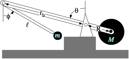
Fig. 2.1.1 An elementary ground-fixed trebuchet
Galileo's failure would have been quite understandable, as we will see below as we begin to do the problem. The trebuchet (treb-yew-shay), a fiendishly clever double arm catapult shown in Fig. 2.1.1, existed in Europe since around the 10th century and a hand operated version in China since 3000BC. A hundred (or a thousand) years of trial and error is hard to beat, particularly if you haven't even invented calculus yet.
Newton's famous Second Law relating force F, mass m, and acceleration a, was not appreciated until the late 1600's. Using differential equations gives the following. (Recall (3.10) or (7.5) in Unit 1.)
 , (2.1.1a)
This was not an easy thing to do until the 1700's. Multi-dimensional Newton's equations such as
 (2.1.1b)
did not appear until around the 1800's. (Physicist J. Willard Gibbs brought Hamilton’s quaternions in a very simplified form to the US. See Unit 4. Such mathematics was not available to Galileo.)
In spite of this, one may grant Galileo partial credit on the trebuchet problem. It is just a pair of compound coupled pendulums. He is known for the first quantitative analysis of the simple pendulum. Small throwing arm l of the trebuchet acts like a simple pendulum after it has thrown its projectile and the big arm r comes to rest upright. We could speculate that an image something like Fig. 2.1.2 b (if he ever saw it) might have stuck in his mind, an empty cable swinging back and forth after each launch.
As is often told, Galileo observed swinging lamps in a Chapel. He may have been first to note that small-angle simple pendulum oscillation rates depend on length but not mass and similarly for descent rates of bodies dropped from the tower of Pisa (neglecting air drag) if in fact he ever did that.
Any connection seen by Galileo between chapel lamps and business end of the terrible trebuchet is pure speculation. Let's just say he got the first part of the trebuchet problem partially correct. This would be the first step of an analysis, which is the breaking down of a complex problem into idealized but doable parts. Galileo analyzed simple pendulum oscillation indicated in Fig. 2.1.2 b without calculus.

Fig. 2.1.2 Galileo's (supposed) problem
However, to solve the whole Trebuchet Problem, Galileo would have needed to do more than invent vector calculus. The neat Cartesian coordinate equations (2.1.1) are too clumsy to do the job very well. There are two angles θ and φ shown in Fig. 2.1.1. They are the natural ones to describe this machine, but the equations describing their motion don't look quite like (2.1.1). Galileo would need to discover Lagrange's equations for generalized coordinates. Generalized curvilinear coordinates (GCC) will be our first topic.
But, poor Galileo wouldn't have done his complete assignment even if he could have derived the correct Lagrange's equations for the trebuchet and given them to the generals. Instead of thanking or paying him for his efforts, they might very well have just shot him on the spot! Differential equations, by themselves, are quite useless unless you can solve them.
As we will see below, the resulting trebuchet equations do not have easy exact analytic solutions. Often one solves such equations numerically many times to learn something about mechanics. To do this in a reasonable amount of time (such as one semester) one probably needs to use a computer. We call this a solution by synthesis; one makes a synthetic or mathematical model or analog to approximate the real thing. Solution by analysis, on the other hand, is an art of idealizing and approximating the problem in terms of its doable parts. These are topics of Units 2 and 3 that expose Lagrangian and Hamiltonian ideas.
But, once again, poor Galileo! Even if he had Lagrange equations and invented computers with integration routines (another century of work) there is still a missing step needed to finish the trebuchet assignment. Lagrange equations are not in a suitable form for numerical integration. Rather the equations need to be what we call Riemann Equations. (This form, introduced in Chapter 2.4 is a main topic of Unit 3 that redoes a lot of Unit 2 more elegantly. You might find it useful to study both Units in tandem.)
The last step is a small one compared to all the others. However, it may be big enough to discourage descriptions of the trebuchet in standard mechanics books. This omission is particularly embarrassing for physicists (Galileo's predecessors) since mechanical engineers have studied trebuchets in considerable detail by computer synthesis. In 1993 two engineers built a trebuchet at Shropshire that tossed a piano over a hundred meters! (Scientific American July 1995) They pointed out that the trebuchet was also called the ingeneium or "ingenious device." This may be the root of the word engine and engineeer.
Perhaps, the old physicists can be excused for continuing Galileo's 'failure' for another seven hundred years. They may express disdain for such a specialized device. ("It's just engineering! ," they harumph, while drawing another draft of smoke from a smelly pipe.) Now, it is true that the trebuchet became a truly awful weapon when it was used for biological warfare by hurling bodies of plague victims into castles under siege. A younger physicist, after a sip of Perrier, might sniff, "We don't do war machines here anymore!" One may certainly use that as an excuse to beg off. But, such excuses wear thin.
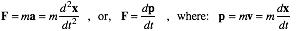
Observant physicists may note the core problem is the motion of the trebuchet which duplicates human throwing, chopping, digging, cultivating, and reaping motions that have been executed billions of times to bring human history and culture to the point where it is now. It was the motion of the scythe that reaped our grandparents’ grain, the swing of the ax that cleared our forests, the arc of the pick that quarried and dug for our buildings, the muscle and hammer that pounded our rail spikes. (See Fig. 2.1.3a.)
In fact, it is probably closer to historical truth to say that it is the trebuchet that mimics the human throwing or chopping motion. It is a human analog. It appears that physicists have, since the beginning of their field, been avoiding discussion of a fundamental mechanical motion that is responsible for building a livable world over countless millennia. The trebuchet dynamics is an old and humanly relevant mechanics that was needed to plant and reap farmers' fields and build both the Old World and the New.
Nowadays power machines do most of our chopping, digging, cultivating, and reaping. Strangely, however, it seems that this has made this particular physics problem even more acutely relevant. In a leisure culture, humans seem unable to stop their chopping, digging, cultivating, and reaping motions, as they become fascinated and habituated to a multitude of lever-sports including baseball, golf, tennis, hockey or lacrosse that mimic these motions. Compare Fig. 2.1.3b to Fig. 2.1.3a above it. Details are in Chapter 7.
Fig. 2.1.3 Trebuchet-like motion of humans. (a) Early work. (b) Later recreation.
The first step in advanced mechanics problems is to choose a convenient set of coordinates to describe the state or position of a system or machine. For the trebuchet the two angles θ and f are sufficient and convenient for locating the moving members relative to the vertical. They do so precisely only to the extent that the cables and beams don't stretch or bend and the base fulcrum is solid and fixed.
For large mechanical systems the bending and stretching is problematic. Some trebuchets had masses of ten or twenty tons and threw 900 to 1300 kilogram projectiles. If the linear dimension or size of a body doubles its mass increases eight times (23=8) with its volume. Meanwhile its ability to resist bending or stretching is proportional to relevant cross-sectional area that only increases four times (22=4) if all its proportions are not altered. Such consideration is called dimensional analysis and should be part of the repertoire of a physicist or engineer. (See Exercises 2.2.1 and 2.2.2.)
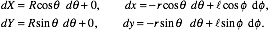
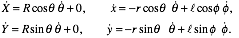
A second step after choosing coordinates is to relate the chosen coordinates to Cartesian coordinates of all masses that will move when the system gets going. The trebuchet in Fig. 2.2.1 has three vectors R, r, and l used to locate masses M and m. The Cartesian coordinates are as follows.
Coordinates of M: Coordinates of m:
X = R sin θ , x = xr + xl = - r sin θ + l sin φ (2.2.1a)
Y = -R cos θ , y = yr + yl = r cos q - l cos f (2.2.1b)
Note that the Cartesian origin has been chosen at the supporting fulcrum, and rotations around this are positive if counter-clockwise. Both f and θ are shown clockwise so they each have a (-) sign. Signs are a major source of errors. Here is a helpful point. Before beginning further calculations you should check that the coordinates are consistent for easily visualized end points. Three such points are shown in Fig. 2.2.2.
Since generalized coordinates are usually non-linear, that is curvilinear, there is plenty of chance for them to become crazy. All curvilinear coordinate systems must have at least one point where they 'go bananas', that is, where they are singular. We'll see more examples of this in Unit 3 where more is said about the topological properties of generalized curvilinear coordinates (GCC).
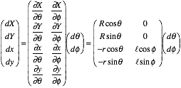
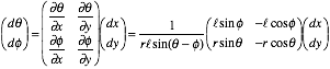
The third step in GCC analysis uses the partial differential chain rule to relate linear differentials of Cartesian coordinates to GCC differentials. For coordinates φ and θ the chain rule is as follows.
 (2.2.2)
From (2.2.2) we get an explicit set of differential relations for (2.2.1).
 (2.2.3)
This shows that the Cartesian coordinates {x,y,X,Y} are not independent variables. There are too many!
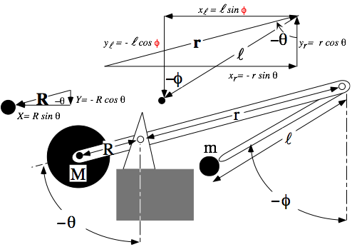
Fig. 2.2.1 Cartesian coordinates related to trebuchet angles θ and φ.
Fig. 2.2.2 Singular positions of the trebuchet.
The object is to see how the Cartesian coordinates will change if we make little tiny changes in one or more of the GCC {φ ,θ }. Not big changes as in Fig. 2.2.2, just tiny ones. This implies that our GCC {φ ,θ } are really independent variables. You can change one or more of them quite arbitrarily without breaking arms of the trebuchet. The same cannot be said for the current Cartesian coordinates {x,y,X,Y}.
For example, you cannot increase X without also changing Y unless you want to break off the R-arm of the trebuchet and void your warranty. An unbroken trebuchet straight from the factory must satisfy a Pythagorean relation of the form
 (2.2.4)
This is an example of a constraint relation. The same goes for Cartesian x and y coordinates of the mass m. However, it looks like x and y are independent because you can imagine grabbing little m like the handle on a swivel lamp and moving it until it reached the limit of the swing. Indeed, x and y are quasi-independent as we will now see. But, they are not independent of X or Y, unless you break the trebuchet in two.
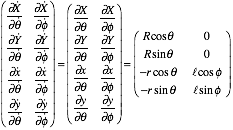
To evaluate dependency one uses Jacobian differential relations. We rewrite (2.2.2) in matrix form.
 (2.2.5)
The rectangular matrix is an example of a generalized Jacobian form. Because it is not square there is no chance of inverting it, that is, expressing dq and dφ in terms of dX, dY, dx , and dy. Well, we know we can't do that without breaking the trebuchet into pieces. But, we might be able to find a square sub-matrix of the Jacobian rectangle that would be invertible.
The first 2-by-2 square is a singular matrix so it won't work. (Recall: X and Y are dependent.)
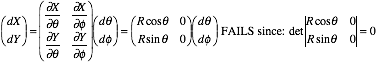 (2.2.6)
However, the last two rows are invertible. (Recall x and y are quasi-independent.)
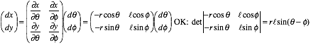 (2.2.7)
The matrix inverse exists if the determinant  is not zero but blows up when
  .
.
 (2.2.8)
That is when the trebuchet is 'stretched out' or 'locked up' as in the first or second of Figs. 1.2.2. At that point x and y can't move independently. Independence fails if the Jacobian matrix inverse fails.
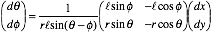
If a Jacobian matrix relation has an inverse, as in the following, it will be called a Kajobian matrix.
 (2.2.9)
The two partial derivative Jacobian and Kajobian matrices are, by construction, inverses of each other.
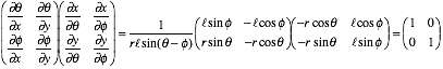 (2.2.10)
Partial derivative chain-rule relations have chain-sums over its quasi-independent x and y variables.
 (2.2.11a)
The matrices commute. (A left-inverse is a right-inverse.) Here the chain sum is over φ and θ.
 (2.2.11b)
This chain-sum is over 'truly' independent φ and θ coordinates. In advanced mechanics one does many such maneuvers that I call 'chain-saw-summing' where a partial derivative is 'sawed' apart and then summed over a set of (supposedly) independent and complete set of variables.
This brings up the question of 'completeness'. Do x and y really provide as complete and reliable a description of the trebuchet as φ and q ? In other words, if I give you x=0.5 and y=2.0, can you tell me what are the values of all the other coordinates, particularly f and q ? By Fig. 2.2.3 the answer is "not quite."
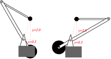
Fig. 2.2.3 Trebuchet configurations with the same x and y
Each GCC manifold has a topology or topological structure that involves its connectivity and maps out its singularities and multi-valued structure. Some more discussion of this is given in Unit 3.
Generalized coordinate differentials lead immediately to generalized velocities. For the trebuchet the velocities follow immediately from the Jacobian chain sums (2.2.2-3). We just 'divide' by dt.
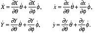 (2.2.12)
The "dot" notation  , etc., for total time derivatives is a nice but only if you write neatly!
 (2.2.13)
There is no need to write new Jacobian relations for velocities. They are identical to the corresponding ones for coordinates. From (2.2.12) and (2.2.13) this leads to what we will call Lemma 1.
 (2.2.14)example
Generalized coordinate acceleration is a little trickier because the curvilinear coordinates give rise to what we call 'fictitious inertial forces.’ Some distinguish 'real' forces such as gravity or a punch in the nose from fictitious ones such as Coriolis effects discussed in Ch. 5 of Unit 1. But, Einstein's famous elevator analogy lends a reality to all inertial forces by noting that the effects may be indistinguishable.
Time differentiation of (2.2.12) and (2.2.13) above gives the following.
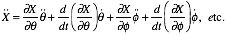 (2.2.15)
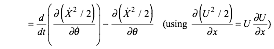
Each variable gives rise to two kinds of terms. First are terms like  that exist even if the Jacobian is constant. Next are terms like
  due to the curvilinear nature of the coordinates. Let us study such time derivatives of Jacobian derivatives using chain-rule sums over independent variables.
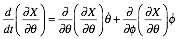
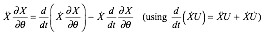
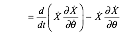
Now φ and θ partial derivatives of X can be done in either order if X is a continuous function of θ and φ.
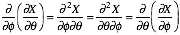
The result (using (2.2.12)) is what we call Lemma 2.
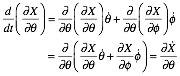 (2.2.16)example
So t-derivative of a Jacobian X coordinate partialθ-derivative is that q-partial of X velocity. (It is pretty hard to say this lemma in words!) Now the two lemmas, Lemma 1 of (2.2.14) and Lemma 2 of (2.2.16) above, will help us write Newton's equations of motion entirely in terms of generalized curvilinear coordinates.
Exercise 2.2.1 This is a dimensional analysis and power law problem. It involves Olympic weight lifters but is a general piece of mechanics that applies to everything. (Have you wondered why toy cars can fall off cliffs without damage while yours cannot?)
Olympic weight lifters are divided into classes according to their body weight. Generally top performers are close to maximum allowed by their class (except for “super-heavyweight" classes.)
(a) From dimensional arguments alone, you can predict that the Olympic records R in a given event (say, the "clean and jerk" which is always the greatest record) should have a definite functional relationship to the weight W=Mg of the performers: R= R(W). Derive R(W) as a power law R=kWp with an undetermined coefficient k.
(b) Obtain a set of records from an almanac or book of records, and plot them against W for a given event or events. See how well your theory and experiment jive. (Hint: It is most convenient to plot on log-log graph paper. Why?)
(c) Use the results of (a) and (b) to answer: How many times his bodyweight could a man lift if he was the size of an ant with a mass of M = 1 gm.? (A real ant is supposed to lift five or ten times its body weight. How much better or worse is the ant doing than "Antman"? )
Exercise 2.2.2Another dimensional analysis problem like Prob. 1.1.1 involves Olympic high jump and animal related capability. A 2 meter jump is considered excellent for a human of dimension L=2m. What are we to expect from equivalent smaller jumpers such as an L=10cm. kangaroo rat or an L=1cm. grasshopper?
How about an L=20m high King Kong? State your arguments.
Conventional classical mechanics starts with Newton's Cartesian F=m equations (2.1.1) as the main classical axiom following momentum conservation (2.1) of Unit 1. They relate acceleration component
  for each mass to a corresponding force component
  Fx , or Fy on that mass due to outside forces and other masses. And, that's a problem. While we know that mass M has a Y-component contribution -Mg due to its gravitational weight and similarly for mass m, the constraint forces on M or m due to connecting arms and ropes are quite difficult to find. Good luck, Galileo!
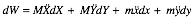
A GCC approach lets us consider only forces that do work. Following (7.5) in Unit 1, the work dW done in a given time interval dt by all the forces on all the masses is a sum of F·dx for all components for all masses. (A general work differential is d(work)=cause·d(effect).) Our trebuchet’s work sum is here.
dW = FX dX + FY dY + Fx dx + Fy dy. (2.3.1)
(We’re ignoring mass of arms.) Now use Newton's equations.
FX = , FY =
 , Fx =
  , Fy =
  (2.3.2)
The work sum then becomes
 . (2.3.3)
These terms lead us to an elegant equation of motion in terms of our generalized coordinates φ and θ and let us ignore unknown (non-causal) constraint parts of Fx or Fy etc.
Substituting the φ and q chain-rule expressions (2.2.2) and (2.2.3) gives the following form for each Cartesian component  . Consider X, first. (The other three are similar.)
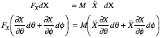 (2.3.4)
Each of the two terms on the right can be expressed as follows.
 (by lemma 1 (2.2.14) and lemma 2 (2.2.16))
 (2.3.5)
Equations like (2.3.4) must be true for arbitrary independent coordinate differentials dφ and dq .
 (2.3.6)
So there are eight equations like these, one pair for each of the four Cartesian coordinates  . But, they still not quite useful by themselves because we don't know the constraint parts of the four force components
  Fx , or Fy , nor can we deal with individual 'partial' kinetic energies like MVX2/2.
However, if we add up the equations like (2.3.6) for all four coordinates  , then the eight equations will boil down to just two. Each involves the total kinetic energy T=KE which is the sum of 1/2mv2 for every moving mass m. For the trebuchet the total kinetic energy is
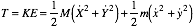 (2.3.7)
(We ignore inertia of arms R, r, and l in Fig. 2.2.1. If arms are massive that is a big mistake! But, we're just getting started here. And besides, those papal-generals aren't paying us enough!)
The sum of equations like (2.3.6) for  is the following very simple pair
 ,
,  (2.3.8a)
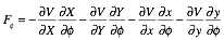
where generalized forces Fθ and Ff are defined as follows. Equation (2.2.14) in lemma 1 was used again.
 (2.3.8b)
=FXRcosθ +FYRsinθ - Fx rcosq - Fy rsinθ = 0 + 0 +Fx l cosφ +Fy l sinφ
These are called the Lagrangian derivative equations. As we will see shortly they are very useful since we do not need to know any forces except those due to gravity or other external influences that actually cause work on the device. Those pesky and unknown constraint forces will cancel out completely, as we will see.
The Lagrangian derivative equations (2.3.8) need a kinetic energy T expressed in GCC  and not in CC
  used by (2.3.7). Jacobian relations (2.2.13) convert velocities of CC-GCC definition (2.2.2).
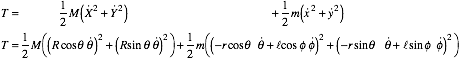
Expanding and simplifying yields the trebuchet kinetic energy KE labeled by T or later by Lagrange’s L.
 (2.3.9)
Note terms of the form Iω2/2 where I=mr2 is a moment of inertia, that is  for the big mass and
  and
and  for the little mass. (Now arm inertia is easy to add to T. See exercise 2.3.2.)
It helps to check and try to rationalize each term that shows up in a Lagrangian algebra.
The last-term ( ) in T is called a Coriolis term or cross term. It is the term that makes the total inertia smaller when the trebuchet has its l-arm tucked under the r-arm. Then φ and θ are equal and the cosine is unity (
 ). Then KE forms
  Iw2 appear with inertia I=mr2.
 (2.3.10a)
The other extreme is the 'stretched out' case when φ and θ are opposite and the cosine is minus unity ( ). Then the total inertia is maximum.
 (2.3.10b)
The intermediate case is when the two arms are orthogonal and the cosine is zero. Then the inertia due to m is just the square of the radial hypotenuse, i.e., a Pythagorean sum  , times the mass m.
 (2.3.10c)
A skater, tucking in his or her arms in order to spin faster, is analogous to the trebuchet. For a given KE (T=const.), angular velocity  will be highest in the 'tucked-in' case-a, lowest in the 'stretched-out' case-b, and in between for the 'orthogonal' case-c.
The concept of orthogonality is important. Let us express the KE as a matrix quadratic form or dynamic metric γμν-tensor sum as shown below. Such quadratic γμν-forms are very important in physics.
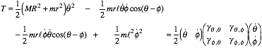 (2.3.11a)
Here the dynamic metric coefficient matrix holds the kinetic coefficients of  in turn.
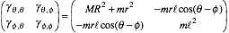 (2.3.11b)
The off-diagonal cross-term coefficients (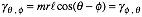 ) are zero if the coordinate lines happen to intersect at right angles or orthogonally as in Fig 2.3.1a. They do this wherever the l-lever is perpendicular to the main beam as in Fig. 2.3.1a where q-f = ±90°. Elsewhere φ and θ curves form affine or non othogonal intersections as in Fig. 2.3.1b. But, this is no problem once we learn to use the γμν’s.
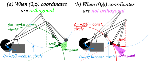
Fig. 2.3.1 Examples of (q,f) intersections (a) othogonal (special case), (b) non-orthogonal (typical).
General curvilinear coordinate (GCC) metrics may not be constant or orthogonal so off-diagonal KE cross-terms
  may be non-zero as in (2.3.9) or (2.3.12a) below. Cartesian KE and metric forms, on the other hand, are simple diagonal
  sums like (2.3.7) or the following (2.3.12b).
 (2.3.12a)
  (2.3.12b)
We shall gain more familiarity with metric tensors  in the following and particularly in Unit 3.
It helps to 'dissect' a GCC KE or quadratic metric form as was done in (2.3.10 a-c). Just as in the analysis of Fig. 2.3.2, this provides a check of the algebra and (after flushing out pesky sign errors) improves one's confidence and understanding of each term.
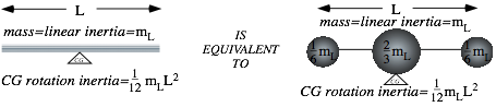
Fig. 2.3.2 Thin symmetric linear lever and its point-mass equivalent.
One may approximate inertial terms for arms and levers without wholly redoing Jacobian relations. This is simplest for linear symmetric arms and levers that are equivalent to a central point mass and two equal point masses on either end as in Fig. 2.3.2. Then the kinetic energy for each of the three mass points is found in terms of the GCC and generalized velocities. (See exercise 2.3.2.)
A general asymmetric body kinetic energy is a bit more complicated and so solid arm inertia requires detailed analysis described in Unit 6.
Exercise 2.3.1Add up all four equations like (2.3.5) or (2.3.6) and verify (2.3.8).
Exercise 2.3.2 Consider some extra terms that might to be added to the trebuchet kinetic energy T and express them in terms of the generalized coordinates θ and φ and their velocities.
(a) Suppose the main big r-R arm had mass MrR and CG rotational inertia I. (Derive CG I in terms of MrR assuming uniform thickness.) Give the extra terms that are needed in T.
(b) Suppose the little l arm had mass Ml and rotational inertia I. (Derive CG I in terms of Ml assuming uniform thickness.) Give extra terms needed in T.
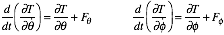
The Lagrange versions (2.3.8) of Newton's equations for the trebuchet are rewritten below.
 (2.4.1a)
These can be viewed as the grand expression of Newton's equations (2.1.1) namely the total time derivative of each component of momentum equals the corresponding component of the total force.
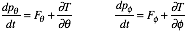 (2.4.1b)
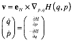
Here generalized momentum is defined like v-derivative (1.6.10a) of Lagrange's velocity dependent L(v)=T.
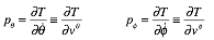 . (2.4.1c)
Each total force ( or
or ) has a genuine part (
 ) and a fictitious part (
 ). Lagrange's GCC equations equate time rate of GCC canonical momentum to total GCC force. It’s just Newton-2 in GCC.
(A "Canon" is law by church or pope. If Galileo had discovered GCC momentum it’s doubtful he would name it in honor of a church that invited him to a barbeque to be the charcoal!)
Here we will compute GCC or canonical momentum components using the KE = T given by (2.3.9).
First we do the momentum θ -component.
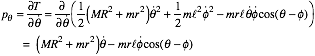 (2.4.2a)
The momentum φ -component is next.
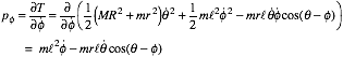 (2.4.2b)
The first term of pq is the angular momentum  of the big r-R arm if
  =0, and the first term of pf is the angular momentum
  of the little l arm if
  =0. The second terms are a little harder to explain, but you can see they give consistent values for the three cases: "tucked-in", "stretched-out", and "orthogonal" that were discussed after (2.3.10 a-c). (See exercise 2.4.1.)
Notice that the generalized momenta (pq , pf ) in (2.4.2) are related to the generalized velocities ( ) precisely through the metric tensor coefficients
  in (2.3.11).
pm=Sgmn , or
, or 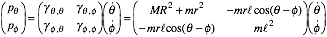 (2.4.3)
The p=g·v relations are a general form and result for GCC systems. (See exercise 2.4.2.)
So far the generalized velocities, accelerations, and momenta have been calculated using partial derivatives. The next to last step in obtaining generalized equations of motion involves total time derivatives and these take just a little more care. Consider first the time derivative  of
of  in (2.4.2a). A dot means total differentiation so everything that moves or can move contributes to it. (It's very easy to miss a term!)
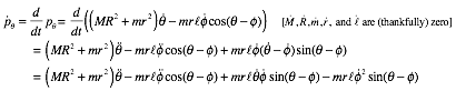 (2.4.4a)
Next, is the time derivative  of
of  in (2.4.2b).
 (2.4.4b)
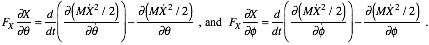
The last step is to calculate the fictitious force term in (2.4.1a), a partial derivative  .
.
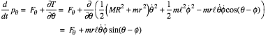 (2.4.5a)
For  the fictitious force term in (2.4.1b) is
  .
.
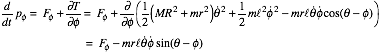 (2.4.5b)
Equating the two expressions above for  and the two expression for
  gives two equations of motion.
 (2.4.6)
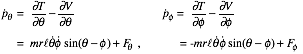
The fictitious force terms have opposite signs. Now recall the 'true' forces from (2.3.8b).
 (2.4.7)
=FXRcosq +FYRsinθ -Fx rcosq -Fy rsinθ , = 0 + 0 +Fx lcosφ +Fy lsinφ .
We need to distinguish externally applied forces like gravity from internal constraint forces due to stress of the supporting arms. Now we see how constraint forces cancel out.
Consider first the constraint force F(m) on the mass m due to little arm l. This force must be along the lever or cable l because its bearing connection to r is assumed to have negligible friction. (If it's just a cable like the original trebuchets it can only pull.) Geometry of Fig. 2.4.1 gives l-constraint force on m.
Fx(m)=-F sin φ Fy(m)= F cos f (2.4.8)
The φ -component of the l-constraint force cancels to zero no matter how large is the tension F.
Ff = Fx(m) l cosφ + Fy(m) lsinφ = -F sin f l cosφ +F cos f lsinφ =0 (2.4.9)
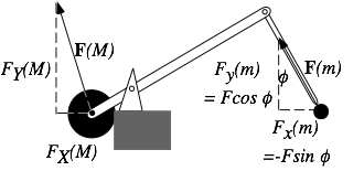
Fig. 2.4.1 Constraint forces on mass M and mass m
Constraint forces FX (M) and FY(M) due to big arm R on mass M are a bit more tricky since F(M) points in whatever direction it needs to in order to keep M at a radius R from the fulcrum. However, the torque on the big R-r-arm due to equal-but-opposite (Newton's 3rd axiom) constraints -F(M) and -F(m) must always sum to zero or the arm's rotation q around the fulcrum will accelerate infinitely since we are still assuming the arm has no inertia. Similarly, the sum of -F(M),-F(m), and F(support) is zero.  (2.4.10a) -F(M)-F(m)+F(support)=0 (2.4.10b)
Hence the constraint forces cancel out of the Fq relation (2.4.7) due to (2.4.10) and do not add to either GCC force component Fq orFf. (See Exercise 2.4.3) The only forces that affect the Lagrange equations are applied forces due to gravitational weight –Mg and -mg
 as shown in Fig. 2.4.2.
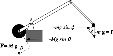
Fig. 2.4.2 Applied forces on mass M and mass m
Cartesian y-components of the applied force are indicated in Fig. 2.4.2.
FX = 0, FY = -Mg, Fx= 0 = fx, Fy = fy = -mg (2.4.11)
These are used in (2.4.7) to give the correct generalized forces.
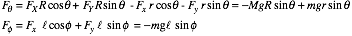 (2.4.12)
This is true even though equations in (2.4.11) are ignoring constraint forces.
Note quantities Fq and Ff are actually not forces at all. They are torques. Note that for positive θ the M-term contributes a negative gravitational torque (clockwise) to Fq while the m term contributes a positive (counter-clockwise) torque because M and m are on opposite sides of the fulcrum. Meanwhile, the mass m contributes a negative or clockwise restoring torque Ff for positive φ.
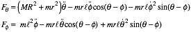
Finally, the equations of motion with only generalized coordinates is the following.
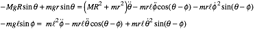 (2.4.13)
Well, the equations are correct but a bit disorderly. Something has to be done to sort them out.
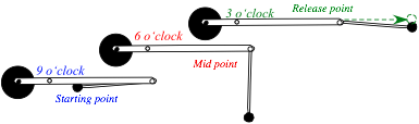
Exercise 2.4.1 Verify that the inertia coefficients of angular momentum in (2.4.2) have the correct m·r2 inertial form for each position: 9 o’clock “tucked-in”, 6 o’clock “orthogonal”, 3 o’clock “stretched out” shown below.
Exercise 2.4.2 If kinetic energy has the metric dummy-index-sum rule form  then verify the canonical momentum formula
  .
.
Exercise 2.4.3 Verify (2.4.10).
Our old friends the metric coefficients γμν from (2.4.3) are hiding in the equations (2.4.13). We rewrite the equations in matrix form in order to expose another important role of γμν metric relations.
 (2.5.1)
By inverting the metric matrix we get an equation with the highest derivatives given explicitly.
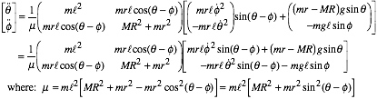 (2.5.2)
Note: the metric determinant m is non-zero even when trebuchet is 'tucked-in' or 'stretched-out'.
The resulting equations are examples of what we call Riemann equations. Most mechanics texts do not include them, but they're quite useful. At the very least, they have a form suitable for numerical integration. More importantly, they lead to relativistic equations of motion. Here, we consider some special cases, generalizations, and approximations. For example, the gravity-free (g=0) equation is as follows.
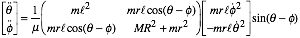 (2.5.3)
Much of advanced mechanics involves competing arts of idealization, generalization, and approximation. A more elegant treatment of Lagrange and Riemann equations is given by Ch. 5 and Ch. 6 in the following companion Unit 3. There we discuss of when and how explicitly time-dependent GCC may be used.
Once again, it is recommended that a new equation be tested for special cases in order to check its algebra and to understand its physics. We're allowed to choose arbitrary values for all independent variables. Let's choose coordinates ( ) and velocities (
 ). This simplifies (2.5.3).
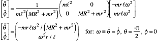 (2.5.3)special case
In the Fig. 2.5.1 below this choice is drawn in order to help assess the resulting forces, torques, and angular accelerations. At this instant the device appears to be rotating rigidly with angular velocity ω.
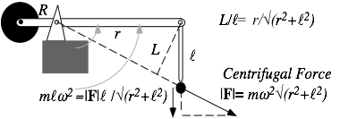
Fig. 2.5.1 Centrifugal force for a particular state of motion (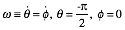 )
)
The f-torque on mass m at the end of leg l due to centrifugal force is the force times moment arm L=r l /√(r2+l2). This is the rate of change of f-angular momentum around the pivot at the top of l.
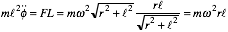 (2.5.4)
This yields
 (2.5.5)
in agreement with the φ-component of (2.5.3). However, it may seem paradoxical that the q-coordinate for the main r-arm should have any torque or acceleration at all. Indeed, if the device is rigid there can be none since the centrifugal force has no moment; its line of action hits the θ-axis of the R-arm.
However, this device isn't rigid. The l-leg pivot is frictionless and can only transmit a component mlw2 of force along l. This causes a negative torque -mrlw2 on the big r-arm. It reduces θ-angular momentum to exactly cancel the rate of increase (2.5.4) in f-momentum, and this agrees with (2.5.3).
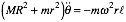 (2.5.6)
Note that, according to (2.4.5) the time derivative of total momentum is zero if outside torques are zero.
 (2.5.7)
Analogy: a twirling skater's body slows down as his or her relaxed arms fly out. This is one way the trebuchet delivers energy to the projectile m, and this will happen even without the help of gravity.
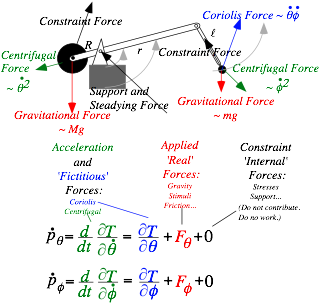
We now pause to review a 'force inventory' associated with the Lagrangian or Riemann GCC force equations. The inventory is sketched in the Fig. 2.5.2 below.
The three classes of forces, acceleration ('fictitious'), applied ('real'), and constraint ('internal') are somewhat arbitrarily named. For example, relativists might regard gravity as an acceleration force. Centrifugal and Coriolis effects introduced in Ch. 11 of Unit 1 are analyzed using different methods in Ch. 7 of Unit 3 where treatment of friction is in Ch. 9. Constraint forces are ignorable if and only if they can do no work. From (2.3.1) we expect no work or energy contribution from constraint forces.
dW = FX dX + FY dY + Fx dx + Fy dy = Fq dθ + Ff dφ = 0 with no applied forces (2.5.8a)
 with gravity (2.5.8b)
This is sometimes called the principle of (no) virtual work.
A geometric reason for ignoring constraint forces is that they always act normal or perpendicular to the coordinate directions. This will be shown more clearly by the GCC tensor geometry of Unit 3. Only forces acting along coordinates φ or θ can accelerate or change their momentum pφ or pθ .
The physics of mechanics is first concerned with net energy and momentum flow in and out of an object and only later with its internal back-and-forth flow, particularly when the latter averages to zero. That is not to say that internal stresses are uninteresting or unimportant! But, to calculate stress it is first necessary to solve for the ideal behavior gotten by ignoring stress. Besides, when an object fails under excessive stress it is the engineer that gets sued and not his physics instructor!
Constraint and stress analysis are addressed from several points of view in Unit 3 Ch. 9 and in Unit 7 discussion of variational methods and in Unit 8 discussion of optimal control theory.
Exercise 2.5.1 Verify (2.5.8).

Fig. 2.5.2 Lagrangian force inventory divides forces into causative real applied forces, inertial accelerative and fictitious forces, and ignorable non-causitive constraint forces.
If theorists can't solve some equations they resort to what they do best: Derive more equations! We do that now before actually solving the trebuchet and related problems. A strategy of 'fighting fire with fire' can show different ways to look at a problem and suggest more elegant solutions.
Many applied forces can be expressed as the gradient of a potential function V.
 (2.6.1)
This is the case for uniform gravitational forces in (2.4.11) for which the potential has a simple form of (mass).(gravity).(height) for each mass. This was first used in (7.6) of Ch.7 in Unit 1.
V(X, Y, x, y) = MgY + mgy (2.6.2)
If a force is a gradient of a potential it is called a conservative force function. As before in (9.5) and (9.8) of Unit 1, we will find that a sum of kinetic energy T and potential V is a conserved constant of motion.
The minus sign in (2.6.1) reverses the gradient vector that points up-slope so a system feels a force pointing down-slope. A positive gradient  is force needed to hold back motion that we called a ‘mathematician-force’ in Ch. 1.7. We mow use a physicist’s-definition
  like (6.9) of Unit 1.
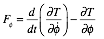
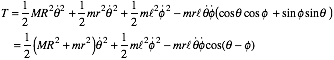
The gradient expression written in generalized coordinates is easy to derive and remember. Recall how we defined the generalized forces in (2.3.8b) as is repeated here.
 (2.6.3a)
Replacing each force by its gradient component (2.6.1) gives the following chain-rule.
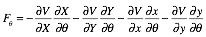
 (2.6.3b)
  (2.6.3c)
This simplifies the formal expression of the Lagrangian force equations (2.4.1a) as repeated below.
 (2.4.1a)repeated
 (2.6.4)
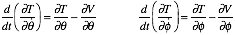
The results are Lagrange's potential equations
 where: L = T - V (2.6.5)
The Lagrangian function L = T - V is the difference between kinetic energy T and potential energy V where (most important!) V(r) is assumed to not be an explicit function of any GCC velocity  variables.

For the trebuchet and related problems the Lagrangian potential equations (2.6.5) represent no computational improvement over the first generalized coordinate equations (2.4.13), and are not as applicable as the Reimann equations (2.5.2). However, they are 'more elegant', that is, they fit in a smaller suitcase. Also, they are just a few steps away from very powerful forms of Newton-equations that are called the Hamiltonian formulations of mechanics.
A Hamiltonian formulation treats generalized momenta and coordinates as independent variables. But, Lagrangians use generalized velocities and coordinates. Differentials of kinetic energy or Lagrangian  are chain rule expansion with a term
  ,
,  or
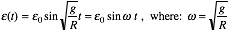
or  for each independent variable. A dt term is needed if there is explicit time dependence in T or V. (For example, an oscillating electric field Ex=E0 sin(w t) has potential V=-E0 x sin(w t) that is an explicit function of time t as well as of position x.)
 (2.6.6)
The total time derivative has the same form as the total differential.
 (2.6.7)
Now Lagrange equations (2.6.5) are inserted while using the identity: 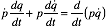
 (2.6.8)
Now we collect the total time  –derivatives on one side and partial
  –derivatives on the other.
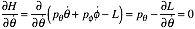
Rewriting (2.6.8) gives or:
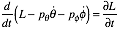
 (2.6.9a)
This is our first explicit Legendre-Poincare relation of the form H=p•v-L after (1.6.11b).
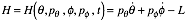 (2.6.9b)
A Hamiltonian function H is constant( ) or conserved (while variables obey the equations of motion) if L has no explicit time dependence (
 ). Metric definition: pm=Sgmn
  from (2.4.3) helps to clarify the form if it is used to expand canonical momentum and the kinetic energy definition in (2.3.11).
 (2.6.9c)
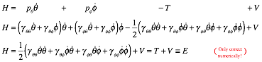
So, the Hamiltonian is the sum of kinetic energy T and potential V that is the total energy E=T+V. Equations (2.6.9) prove the conservation of total energy provided L is not an explicit function of time.
Consider now the explicit or formal dependence of the Hamiltonian H. The definition (2.6.9c) is correct numerically, but not formally. Rather, Hamilton intended to express H in terms of generalized coordinates and momenta only. No explicit velocity dependence is allowed. So let's express  in terms of
  using inverse metric coefficients gmn first derived for the Riemann equations (2.5.2).
 (2.6.9d)
Here are the gmn-metric relations again from (2.3.11b) and the inverse gmn-relations.
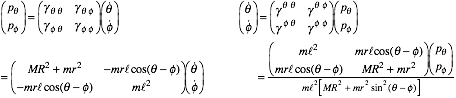
(2.6.10a) (2.6.10b)
The partial derivative of the Hamiltonian H with respect to a generalized velocity is formally zero. So is the formal partial derivative of the Lagrangian L with respect to momentum. (Recall (1.12.6) in Ch. 12 Unit 1.)
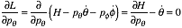 (2.6.11a) (2.6.11b)
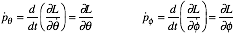
The former (2.6.11a) defines momentum (again). The latter (2.6.11b) is a 1st type of Hamilton's equations.
 (2.6.12)
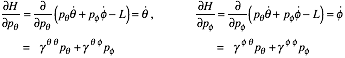
The 2nd type of Hamilton's equations involves partial derivatives of H with respect to coordinates.
 (2.6.13a)
These yield equations that are numerically the same as Lagrange's equations (2.4.5).
 (2.6.13b)
However, to make them strictly conform to explicit Hamiltonian form, the generalized velocity factors in the above (2.6.13) must be expressed in terms of momenta and coordinates only. You should work out these expressions. (See exercise 2.6.1.) Below is a summary of our examples of Hamilton's equations.
 (2.6.14)
The Hamiltonian form (2.6.14) of Newton's equations is regarded as a crowning achievement of classical mechanics. Indeed, the Hamiltonian formalism is the steppingstone to a number of powerful theoretical generalizations including the development of quantum mechanics.
However, at first sight they don't seem to help the trebuchet generals much. Galileo would not have made them very happy even if he had gotten this far. The equations have a deceptively simple first-order form, but we have seen that the emphasis is on the word 'deceptively'; at first, they are really no easier to solve numerically than the earlier Lagrangian or Riemann forms.
However, one of the advantages of the Hamiltonian formulation has already shown itself; it suggests conservation laws. We have seen that absence of explicit time dependence implied energy conservation; or more precisely, that the Hamiltonian H was a constant of the motion.
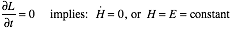 (2.6.15)
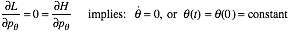
By analogy we see that the absence of explicit coordinate dependence (suppose that the Hamiltonian H was not a function of θ at all) leads to momentum conservation. (By (2.6.14) angular momentum is constant.)
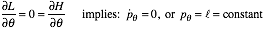 (2.6.16)
Hamilton's equations show the beautiful relation between symmetry in a generalized coordinate like q and conservation of its conjugate momentum pq. Symmetry, in this case, means that the system 'looks the same' for all values of the coordinate q or is invariant to changes of that coordinate. In other words, we find no 'lumps' so the Hamiltonian doesn't go up or down as the symmetry coordinate θ moves. Because of this symmetry or 'smoothness', the system cannot alter momentum belonging or conjugate to this coordinate.
In other words: "No lumps means no bumps!"
The concept of conjugate or canonically conjugate variables, such as pq and θ or pf and φ, is important to Hamiltonian mechanics. A pair of variables (q,p) that satisfy a pair of Hamiltonian equations
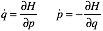 , (2.6.17)
are said to be canonically conjugate with respect to Hamiltonian H. By a similar definition one may say that total energy and time  are also a conjugate pair of variables.
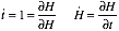 (2.6.18)
However, the ±sign difference amounts to a big distinction between spatial coordinate variables like(pf,φ) and temporal or time-like variables (t,H). This is at the heart of relativistic invariance and quantum theory.
The difference for the (H,t) pair is the sign of the second equation. Time and energy, while analogous to position and momentum, are also distinguished by their respective places in the Lagrangian differential.
 (2.6.19)
This is called Poincare's invariant, or the differential of action S. It is an important form in physics, and we shall discuss it often. Note for now that S has the form of relativistically invariant phase k•r-wt in a plane wave  . (Laws of Planck (E=hw) and DeBroglie (p=hk) are being invoked here.)
 (2.6.20)
Relativity and quantum theory are deeply connected to Hamiltonian mechanics.
Momentum independence of a Hamiltonian has implications analogous to coordinate independence or symmetry. It implies that the conjugate coordinate cannot move; it's just a fixed parameter.
 (2.6.21)
In other words: "No energy for momentum means no-go!" An active coordinate qm must have at least one term in H containing its conjugate momentum pm. Otherwise it’s just a dried-up constraint qm=constant like the trebuchet arms R or l that (our approximation assumes) are constraints that cannot change.
Constraints are what keep our classical devices together and it is a good thing if and when they can be treated as constants. How far would we be on the trebuchet problem if its Hamiltonian were a function of every nut, screw, and wood molecule in the machine? We wouldn’t be much better off than Galileo trying to satisfy his generals and popes!
Idealization by constraint, particularly, frictionless constraints, is one of the keys to a successful Hamiltonian or Lagrangian mechanics. Now we consider some idealizations of the trebuchet that simplify it to a pendulum. (Also, this provides one more algebra check.)
Exercise 2.6.1Verify or finish Hamilton’s equations for trebuchet (2.6.10) thru (2.6.13).
Exercise 2.6.2Elementary application of Lagrange or Hamilton equations.
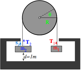
Consider a bicycle chain of fixed length l draped over a pulley or sprocket of radius R =0.5m. and holding up two masses m1 =1kg. and m2 =2kg. Chain cannot slip relative to pulley even if one of the masses breaks free. Pulley is a circular disc of uniform density and mass M=4kg. and radius R =0.5m. and rotates freely. Initially, a string under tension S2 keeps mass m2 from moving as shown. Constraint forces on bicycle chain are indicated (not to scale) by T1 and T2 . At t=0 the string is cut.
Before stringS2 is cut (t<0).
(a) Give the magnitude of the forces T1, T2 and S2 .
(b) Give the magnitude of the rotational inertia of the disc.
After string S2 is cut (t>0). Let gravity acceleration be exactly g=10 m/s2.
(c) Give Lagrangian and Lagrange equations in terms of angle q of the disc rotation.
(d) When does mass m2 hit bottom?
(e) Between string cutting and mass m2 hitting bottom, compute force magnitudes T1 and T2 .
Suppose mass m1 or m2 falls off its chain if its force exceeds Fbreak (but they don’t break simultaneously.)
(f) Which mass (or masses) may break free if Fbreak = 20N.?
(g) Which mass (or masses) may break free if Fbreak = 30N.?
(h) Which mass (or masses) may break free if Fbreak = 15N.?
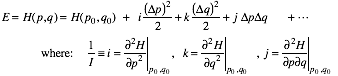
Let us look at Galileo's original problem: a swinging pendulum like the one in Fig. 2.1.2 after the trebuchet has thrown away mass m. Since our model assigns no mass to the throwing leg l we will, instead consider the large R-arm pendulum holding the massive counterweight M. In other words we will just set m=0 in all our trebuchet equations. The pendulum Hamiltonian then follows from equations (2.6.9).
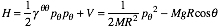 (2.7.1a)
The gravitational potential of the remaining counterweight mass M follows from (2.6.2).
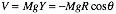 (2.7.1b)
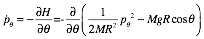
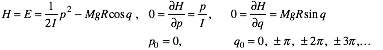
Then Hamilton's equations (2.6.14) are the following.
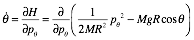
 (2.7.2a)
  (2.7.2b)
Hamiltonian theory might be regarded as overkill for such an elementary system. Newton, Riemann, or Lagrangian forms give the same coordinate equations we get by combining the Hamiltonian pair above.
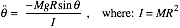 (2.7.3)
This is the coordinate equation for the general compound pendulum of inertia I whose center of mass lies at radius R from the pivot point. For a simple pendulum (point-mass on a massless stick), mass M drops out.
 (2.7.4)
For small swing angle the sine is nearly equal to its angle in radians. ( )
)
 (2.7.5)
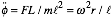
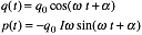
This is a small oscillation approximation, which gives a simple harmonic oscillator equation.  (2.7.6)
Its solution  has angular frequency w (frequency n).

 (2.7.7)
It is the same for arbitrary values of initial phase a or any small values of the oscillation amplitude A.
However, for larger amplitudes the solution is more complicated. But, because the H=E is constant by (2.6.15) we can express the momentum in terms of the angle and total energy E.
 (2.7.8)
Then Hamilton's first equation leads to a (deceptively) simple differential equation.
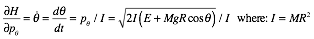 (2.7.9)
Pendulum geometry in Fig. 2.7.1 describes force, energy and time. Torque Fθ equals -Mg·x exactly but potential Mg·h only approaches Mgx2/R at low x. V=MgY is non-linear inq with zeros at q=±p/2.
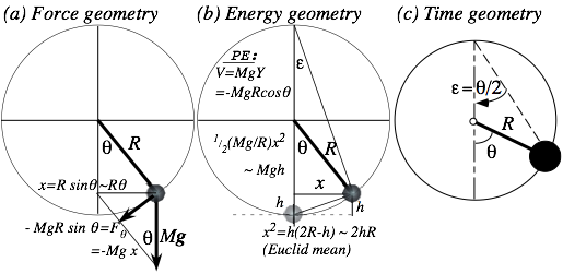
Fig. 2.7.1 Simple pendulum geometry for (a)Force, (b) Energy, (c) Time. e= q/2 defined.
Suppose the pendulum is released at initial angle q0 where potential energy is  . This PE must be the conserved total energy if initial velocity and kinetic energy are zero.
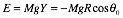 (2.7.10a)
This lets us integrate (2.14.9) between θ0 and 0.
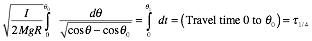 (2.7.10b)
This is known as a solution by quadrature or, in plain English, by an integral over a quarter period. The name refers to the time it takes the pendulum to go between its maximum amplitude and origin (or vice versa) that is one-quarter of a complete back-and-forth oscillation, or a quarter period t1/4 in duration.
A standard form for the integral uses a half-angle coordinate e = q/2 shown in Fig. 2.7.1.
 .
.
A standard quadrature formula follows using d q=2de.
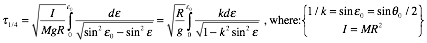 (2.7.10c)
The integral is known as an elliptic integral of the first kind: F(k,e0)=am-1 or the "inverse amu" function.
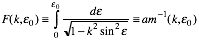 (2.7.10d)
Integrals related to F(k,e) pop up in many mechanics and electromagnetism problems. Many tables of them exist, and most general-purpose computer routines include a library of elliptic functions.
Elliptic integrals simplify in the small-vibration case when a sine function nearly equals its argument. ( as in (2.7.5)) Then the elliptic integral reduces to an elementary one.
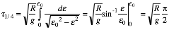 (2.7.11)
The quarter period  is, indeed, one quarter of the simple pendulum period
  . (Recall (2.7.7).) The integral can also give the complete time behavior as an inverse sine function.
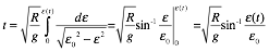 (2.7.12a)
The inverse of this is the usual sine wave solution to (2.7.6).
 , (2.7.12b)
(Either angular coordinate, ε or θ, satisfies this.) But, large-vibrations require Jacobi elliptic functions or "amu" functions. Also defined: "snu" and "cnu" functions sn and cn.
 (2.7.13)
For higher swings as ε0 approaches π/2 (or θ0 approaches π) the period (2.7.10c) of the "amu" function grows, approaching infinity when the pendulum tries (vainly) to "stand on its head."
For energy beyond the q0 =±π point, a pendulum will stop swinging and loop around and around like a high bar gymnast. Visualizing pendulum vibration or libration (swinging) and rotation (looping) is best done using a Hamiltonian phase portrait. This is a plot of possible trajectories in the space (pq, q) of momentum-vs-coordinate angle that is called phase space. For the pendulum this is just a plot of (2.7.7) for various constant values of energy H=E. Resulting phase paths are plotted below.
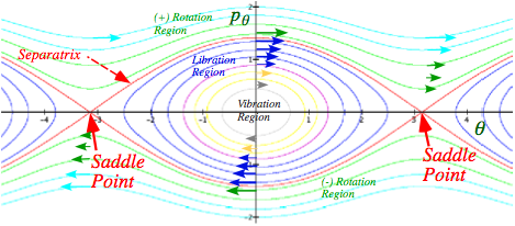
Fig. 2.7.2 Phase portrait or topography map for simple pendulum
Fig. 2.7.2 is a topography map for the Hamiltonian H(pq q) in phase space. A 3D plot of the Hamiltonian topography is shown below in Fig. 2.7.3. If you were to slice a horizontal plane parallel to the (pq q) phase plane but at altitude H=E, then its intersection with H(pq q) mountains or valleys would be one of the constant-E paths in Fig. 2.7.2. These topo-E-level curves are seen in Fig. 2.7.3, too.
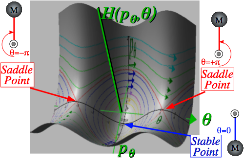
Fig. 2.7.3 Hamiltonian H(pq,q) topography plot for simple pendulum
If the energy is low (E<MgR ) then the phase path in Fig. 2.7.3 will be an oval going around a valley and doing pendulum vibrational or librational motion. If the energy is high (E>MgR ) then the path will be wavy line doing pendulum rotational motion along a high mountain road to the right (counter-clockwise rotation) or else to the left (clockwise rotation). The dividing path at energy (E=MgR ) is called the separatrix (curve that separates) between these two types of motion. The two branches of the separatrix meet at so-called saddle points on top of the mountain passes in Fig. 2.7.3 where the pendulum is "standing on its head."
Hamilton's equations can be viewed in phase space as a "cross-gradient" in the following form.
 (2.7.14)
The velocity vector in phase (q,p)-space is proportional to the gradient or slope of H at each point but is directed perpendicular to the fall line. In ordinary (x,y) space it is the acceleration or force vector that is proportional to the gradient of the potential V and is directed down the fall line.
Phase plots often look a little like storms drawn on a weather map. The one in Fig. 2.7.2 looks like the Jovian "red spot", a fierce storm on Jupiter. A sailor or pilot might use a weather map to locate the quietest areas or "eyes" of the storm and steer toward them. In phase plots these "eyes" surround what are called fixed points in a phase plot.
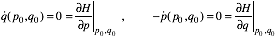
Fixed points (q0, p0) are the points where both the coordinate and the momentum stand still. Examples of fixed points in Fig. 2.7.2 are the two saddle points at p0 = 0 andθ0 = ±π and a stable point at p0 = 0 andθ0 = 0. These special points are also indicated in the 3D plot of Fig. 2.7.3, and they are just the level points where the gradient of the Hamiltonian is a zero. Then
  and
and  are zero, too.
A Taylor expansion of a Hamiltonian function H(q,p) can be done around any point (q0 ,p0) in phase space for which H(q,p) is properly defined. Let H(q0,p0) be H0 and set: <Δq=q-q0 and: Δp=p-p0.

Linear terms at fixed points must be zero according to Hamilton's equations. (2.7.15a)
 (2.7.15b)
For small deviations (<Δq,Δp) around fixed point (q0 ,p0) the Hamiltonian is a quadratic form in (Dq,Dp).
 (2.7.16)
The pendulum Hamiltonian (2.14.1) has the following fixed-points by equations (2.16.1b).
 (2.7.17a)
The first fixed point (q0,p0)=(0, 0 ) has the following elliptical quadratic form.
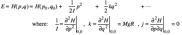 (2.7.17b)
For fixed values of E these are equations of ellipses ( Ap2 + Bq2 =1 ) in phase space. (See Fig. 2.7.4a)
The other fixed points (q0,p0)=(0, ±π ) have the following hyperbolic quadratic form. Let: Dq=q-p .
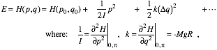 (2.7.17c)
For fixed values of E these are equations of concentric hyperbolas ( Ap2 - Bq2 =1 ). (See Fig. 2.7.4b)
Elliptic points lie at the center of a region of stable vibrational motion, which, near the elliptic point obey Hamilton's equations for an approximate Hamiltonian (2.7.17b) for simple harmonic motion.
 (2.7.18a)
Circular sine or cosine solutions (Recall (2.7.12b)) are small-amplitude-vibration approximations.
 (2.7.18b)
Angular frequncy ω is independent of amplitude  only for the small
  . If
. If  is made larger, then this solution, like that of the pendulum (2.7.12b) for larger
  , may become less and less accurate.
Hyperbolic points lie at the center of a region of unstable motion, which, near the hyperbolic point, obey Hamilton's equations for an approximate Hamiltonian (2.7.17c) for exponential "blow-up."
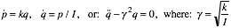 (2.7.19a)
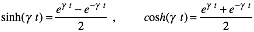
The hyperbolic sine or cosine function solutions are small-amplitude-growth approximations.
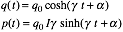 (2.7.19b)
But, even a small amplitude  may grow exponentially and eventually invalidate the approximation. This describes the time behavior on hyperbolic paths near saddle points (q0,p0)=(0, ±π ) in Fig. 2.7.2. Note that the solutions (2.7.19) have both positive and negative exponentials. So q(t) may "blow down" at first.
But, after awhile the positive exponentials generally win and finally q and p have to "blow up." An exception to this involves motion exactly on a separatrix or hyperbolic asymptote. However, such motion is very sensitive to error or noise both classical and quantum. (See problem 2.16.1)
The cross term jpq in (1.16.2) is zero for the pendulum example in Fig. 2.7.2. A cross terms gives tipped or rotated elliptic (or hyperbolic) paths as noted after (1.11.20) in Unit 1. (Recall Exercise 1.11.1.)
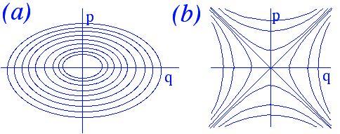
Fig. 2.7.4 Phase paths around fixed points (a) Stable point (b) Unstable saddle point
Pendulum phase flow in Fig. 2.7.2 is given by  if
if  denotes phase space
 in (2.7.14).
 (2.7.14)repeated denoted by:
  (2.7.20)
This velocity flow has zero divergence ( ) since an xy-partial is symmetric to order. (
 =
= )
)
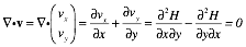 (2.7.21)
On the other hand, the curl( ) of this pseudo-velocity field is (-)the Laplacian div-grad of H(x,y).
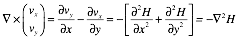 (2.7.22)
For an HO Hamiltonian (H= mp2+
mp2+ kq2) the curl works out to be a constant
  for a rigidly rotating HO phasor-space or rotating A-field (2.8.15) of constant
  in Fig. 2.8.1. Global properties of v-fields are revealed by Gauss divergence –flux or Stokes curl-circulation integrals (2.7.23). The first is total flux
 across a closed contour C around area A along its normal
  , and the second is the integral of v-circulation
 along its tangent to contour C. Total flux (circulation) is A -integral of
  (
( ).
).
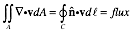 (2.7.23a)
 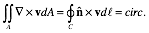 (2.7.23b)
By (2.7.21) total flux is zero for any (q,p)-phase-space area A. The v-flow is that of an incompressible fluid whose density r is time constant as guaranteed by the flow continuity equation, itself a relativistic invariant.
 (2.7.24)
Crowded (q,p)-phase paths in Fig. 2.7.2 represent increased traffic velocity and not an increase in density r of points, and vice versa, lack of crowding at saddles is due to more loitering and not to any change in r.
Indeed, if three or more points define a (q,p)-phase-space area A, then as all the points in A follow their respective phase-paths the area they enclose is supposed to remain constant even as A becomes very distorted. This Liouville Theorem is quite a claim. It might appear we need a proviso that A has no singular points where  is undefined such as at pendulum saddle points in Fig. 2.7.2, but apparently not!
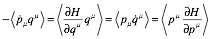
Phase space products like p·q or  may or may not be constant, but average p·q-values of bound orbits over one or more periods tend toward constant or zero values. For example, oscillation q=asinwt and p=bcoswt has a phase product p·q=absinwt·coswt=
 absin2wt that averages to zero. So, it is reasonable to posit a zero value for the time derivative of average p·q-values
  . (
. ( denotes a time average of x.)
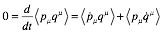 (2.7.25)
Hamiltonian H=T+V and Lagrangian L=T-V relate by to give a virial relation of work to KE=T.
 (2.7.26)
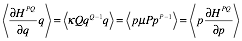
Hamilton equations  and
and  (2.6.14) give virial relations of kinetic KE=T to potential PE=V.
 (2.7.27)
Virial relations take a simple form for a power-law Hamiltonian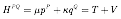 .
.
 (2.7.28)
The resulting virial theorem shows the average ratio KE:PE is inverse to their power ratio  .
.
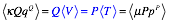 (2.7.29)
Q:P ratios for Coulomb orbit (-1:2), harmonic oscillator (2:2), 4th-power well (4:2), and square well (∞:2) are consistent with what one expects. The latter is 100% KE. A d-dip potential V(x)=- d(x) is 100% PE.
Approximate quantum energy levels are given in terms of an action quantum number u =p·q/h by minimal HPQ-values subject to an uncertainty constraint p·q=hu=const. Recall (1.6.14) in Unit 1. We set q=hu/p and find root pMIN of the HPQ derivative with respect to p that will give minimal HPQ.
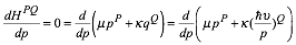 has root:
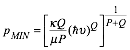
Substituting the root pMIN into the constrained HPQ function gives energy levels as function of u.
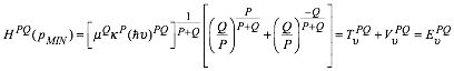 (2.7.30)
Kinetic coefficient m=1/2m and power P=2 are standard. Coulomb PE uses Q=-1. Oscillator uses Q=2.
 (2.7.31a)
 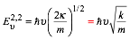 (2.7.31b)
So (2.7.30) approximates quantum Bohr-Rydberg-Coulomb and Planck oscillator (for k=k/2) levels.
Exercise 2.7.1This is another dimensional analysis problem with a power-law (L)p solution. Consider what the walking or strolling speed is for a legged animal if its legs are half its height L. Suppose it strolls by swinging its nearly-free pendulum legs. (Forced oscillation may be the subject of a similar problem in Unit 4.) Limit the swing to Dq=±15° so we may assume harmonic oscillation.
More advanced problem. Discuss how walking speed might vary with larger (anharmonic) stride range |Dq|>15°. First, discuss how pendulum frequency begins to decrease with Dq and so does the increase in stride length as lcos |Dq|approaches l. Show these dynamic and geometric effects lead to an optimal stride and speed.
Many mechanics problems are “gizmos” that model some principle(s). Here are two important examples.
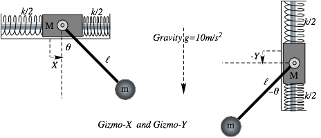
Exercise 2.7.2 Suppose a main mass M slides on the beam attached to Earth by springs with total Hooke-constant k and carries a simple pendulum mass m on a frictionless lever l. Consider two such devices, one horizontal (Gizmo-X) and one vertical (Gizmo-Y).
(a) Derive the Lagrangian equations of motion for the devices.
(b) Derive the Hamiltonian equations of motion for the devices. Identify any constants of the motion.
(c) Reduce the equations to approximate small vibrations.(|θ|<<1,|X|<<1,|Y|<<1)
(d) Reduce equations (a) for the case that M>>m but let k/Mand g/lbe comparable values.
Exercise 2.7.3 Suppose the main trebuchet driving mass M could slide on the beam but was held by a spring of Hooke-constant k at an equilibrium radius R0 at resting angle q=0. Describe how the equations of motion change to describe such a device.
(a) First, give equations with no second mass m and no gravity g.
(b) Then add gravity g.
(c) Then add the projectile mass m on lever l.
Exercise 2.7.4Check the derivation of the power-law potential virial ratio (2.7.29) and fixed-action minimum “quantum” energy (2.7.30). Discuss <KE>/<PE> ratios of average potential and kinetic energy for the most common potentials including the (ion-atom) inverse quadratic power law potential V(q)=k/q2. List formulas for “quantum” energy levels derived in this way for common potentials square (V=kr∞), HO, Coulomb, atom-ion V=ar-2, and delta (V=-kr-∞)). Can the method work for logarithmic potentials? …for non-integral power law potentials? Discuss.
Newton's equations combined with Maxwell's definitions for electromagnetic fields can be put in Lagrangian and Hamiltonian form. This is based upon the so-called pondermotive form for Newton's F=ma equation for a mass m of charge e. The electron charge e=-1.602176Coulombs is imagined here.
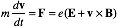 (2.8.1)
First, the electric field E and the magnetic field B are expressed in terms of scalar potential field F=F(r,t) and a vector potential field A=A(r,t) as follows.
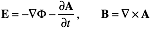 (2.8.2)
Combining these gives a  double-cross term.
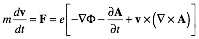 (2.8.3a)
The double-cross is unraveled by Levi-Civita’s identity in Appendix 1.A.
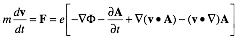 (2.8.3b)
A chain rule expansion of the vector potential total t-derivative is then used.
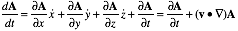 (2.8.4)
Combining this with (2.8.3b) allows a Lagrangian form (2.6.4) to emerge.
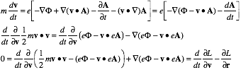 (2.8.5a)
The resulting Lagrangian has a linear velocity term ev•A in addition to the usual quadratic KE=mv2/2.
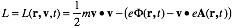 (2.8.5b)
The canonical momentum is defined by L’s v-derivative according to (2.6.5)
 (2.8.5c)
Without the magnetic vector potential A=A(r,t) the Lagrangian has the usual form L= T - V in (2.6.5) with a electric (scalar) potential V=eF(r,t) . However, the vector potential term -v.eA leads to an unusual canonical momentum p. Particle momentum mv is not canonical, but related to canonical p as follows.
 (2.8.6)
The Hamiltonian function of the Legendre-Poincare form defined in (2.6.9b) is the following.
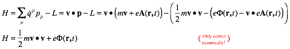 (2.8.7)
Interestingly, the vector potential A seems to cancel out completely, leaving a familiar H=T+V form seen first in (2.6.9c). However, the Hamiltonian is formally correct only if it is written in terms of canonical momentum, not velocity. Just like (2.6.9c), the equation (2.8.7) above is numerically correct, only. Using (2.8.6) to rewrite velocity v in terms of momentum p gives the following.
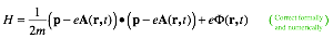 (2.8.8)
The result expands into a more complicated but still formally correct Hamiltonian.
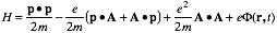 (2.8.9)
Hamilton's equations (2.6.14) then follow. The  equation just relates
  to p. (Recall (2.8.6).)
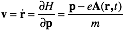 (2.8.10)
For the  equation we use index notation to avoid confusing
 and
and  .
.
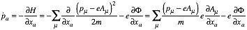 (2.8.11a)
We use (2.8.2) to express F in terms of E and A, and (2.8.10) to give p in terms of v.
 (2.8.11b)
Index notation for (2.8.4) is
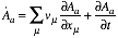 (2.8.12)
Finally, an equation for particle momentum is found by combining the preceding two equations.
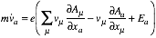 (2.8.13)
The result cancels out the partial time derivative of the vector potential A, and is the same as the simple Newtonian equations (2.8.1-3). The Lagrangian and Hamiltonian forms have no obvious advantage, here. If you just need Cartesian equations of motion, Newton will usually win! However, the Hamiltonian form may win in other coordinate systems if the question of conservation laws and symmetry arises.
Consider how a particle orbits in a constant electric field E which is perpendicular to a constant magnetic field B . A constant E field has a scalar potential field F with constant gradient.
 (2.8.14)
A constant B field has a vector potential field A that resembles the velocity field of a disc or body spinning counter-clockwise around the B axis. (See Fig. 2.4.1.)
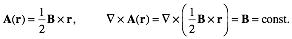 (2.8.15)
Suppose the B field is along the z-axis while the E field is along the x axis as in Fig. 2.8.1. Many effects of arbitrary B and E fields can be seen if we first understand this one.
The Newtonian electromagnetic equations of motion (2.8.1) are repeated here.
 (2.8.16a)
The Newton equations are given explicitly below for the fields (2.8.14) and (2.8.15).
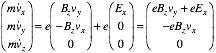 (2.8.16b)
The reduced (x,y) velocity equations are

 . (2.8.17)
Note z-velocity is a constant. These are made into second order oscillator equations with solutions.
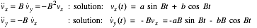 (2.8.18a)
So the vx equation gives simple harmonic motion at the cyclotron angular frequency w c=B=eBz/m while the vy equation gives simple harmonic motion plus an integration constant that is a y-ward drift velocity.
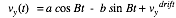 (2.8.18b)
The drift velocity is found by substituting (2.8.18) into (2.8.17).
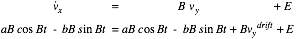 (2.8.18c)
The substitution checks only if the following holds.
 (2.8.18d)
So, a positively charged particle would drift downward in Fig. 2.8.1 perpendicular to the E field while spiraling around the B field. This is analogous to the Hall-Effect drift in conductors.
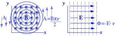
Fig. 2.8.1 Crossed magnetic and electric fields and their potentials
Now we integrate the velocity equations to get the coordinate positions at time t.
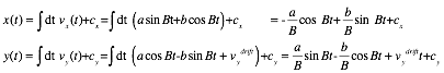 (2.8.19)
At an initial time t=0 the integration constants may be related to initial conditions:
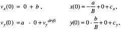 (2.8.20a)
Solving for coefficients a, b, and (cx, cy) gives revealing forms of rotation matrices and vectors.
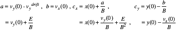 (2.8.20b)
The velocity vector from (2.8.18-8) reduces to the following rotation plus translation.
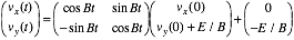 (2.8.21)
Velocity v(t) is a rotation Bt clockwise (for B=eBz/m>0 ) of initial vector v(0) plus a constant drift downward (for E=eEx /m>0 ) of velocity -E/B. The position r(t) vector (2.8.19) is similarly viewed.
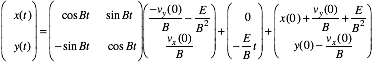 (2.8.22)
Examples of trajectories for fields (E=1/2 , B=1.0) are shown in Fig. 2.8.2. These all correspond to points on a rolling "railroad wheel" as shown in Fig. 2.8.3. First let us zero the initial velocity to v(0)=0 in (2.8.22) so it simplifies. This corresponds to the trajectory in part (a) of Fig. 2.8.2.
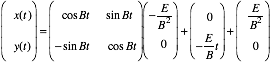 (2.8.23)
The point (x(t),y(t)) sits on the rim of a wheel of radius R=E/B2=1/2 rotating at w c= B=1.0 while the wheel's center drifts along at velocity vdrift =-E/B=-1/2 down the Y-axis. In one cyclotron orbit period tc=2π/B, (here tc=2π), the wheel revolves once and drifts a distance equal wheel circumference 2πR.
y=vdrifttc= -(E/B)2π/B=-2πE/B2=-2πR=-π (2.8.24)
The wheel rolls without slipping on the Y-axis, and the (x(t),y(t)) trajectory is a simple cycloid as shown in Fig. 2.8.2a. Points on a rolling rail wheel make other trajectories, too. However the trajectories will be curlate cycloids if the particle sits on a rim whose radius Rrim is greater than Rw of the wheel in Fig. 2.8.3, or else prolate cycloids if the particle is at a radius less than Rw. The rim vector is the operand in (2.8.22).
rrim(0) = (-vy(0)-E/B , vx(0) )/B (2.8.25)
In order to use the picture we need a formula for the radius Rw of the wheel. This is just the point where the velocity w cRw due to cyclotron rotation exactly cancels the constant drift velocity  .
.
 (2.8.26)
So all the trajectories in Fig. 2.8.2 have the same sized wheel, but most of the ones shown in Fig. 2.8.3b and all but one of the paths in Fig. 2.8.3c have a larger rim radius |rrim|> Rw.
The latter are obtained by throwing the particle along the x-axis in the direction of the electric force. Like a boomerang, it always loops back and forth across the y-axis while drifting down it at a rate determined by the Ex field strength. Without the E-field, the path is just a cyclotron circular orbit.
To make prolate or “loopless” cycloids one must throw the particle down the y-axis. If the vy(0) speed is just right, the path is the “most-loopless” cycloid, that is, a straight line! Then the static electric eEx-force just balances the  component of the magnetic field.
Have trouble remembering directions of 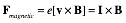 ? Then here is a “right-hand rule” with political overtones that won’t let you easily forget it. The FBI is, rightly or wrongly, thought of as a right-wing organization. Right? Well, take your right hand and write (right) the letters “F”, “B”, and “I” on the right-most three fingers as your hand faces you with the “I” on the thumb (at the right, of course).
Finally, make a “gun” (FBI uses guns, right?) with the fingers of the right hand extended naturally perpendicular to each other. This gives directions of force F due to magnetic field B acting on current I=ev due to a positive charge e traveling along velocity v. (PS: Don’t let the NSA see you doing this!)
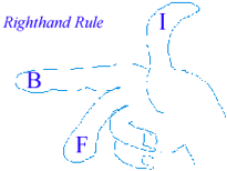
(a) vx(0)=0, vy(0)=0 (b) vx(0)=0, vy(0)=-2 to 2 (c) vx(0)=0 to 2, vy(0)=0
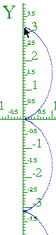

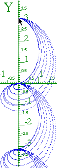
Fig. 2.8.2 Trajectories of unit charge and mass in magnetic and electric fields (E=1/2, B=1)
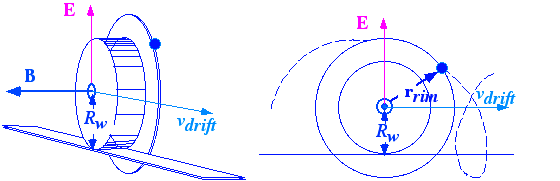 Fig. 2.8.3 Rolling railroad wheel and rim analogy for cyclotron orbits
A smooth sphere or ball rolling on a horizontal rotating table, as shown in Fig. 2.8.4 obeys the same equations as a charged particle in a uniform magnetic B field (and E field if the turntable is tilted).

Fig. 2.8.4 Mechanical analog of magnetic v¥B cyclotron mechanics.
A plastic pool ball has linear velocity as it rolls without slip at angular velocity ω(t) on a plexiglass® disc turntable turning at constant angular velocity W = W
 . The velocity vector of the ball bottom contact point (v(t)-ω(t)¥R) must equal the table surface velocity W¥r(t) at its contact point r(t).
v(t)-ω(t)¥R= W¥r(t) (where: R=R and W = W
 are constant.)
 (2.8.27)
Newton-2 for translation is Force= , and for rotation it is
 as in Fig. 2.8.4.
 (2.8.28)
The acceleration  is given by the time derivative of the velocity constraint (2.8.27).
 (2.8.29)
Putting in (2.8.28) gives the velocity equation of translational motion on the table.
 (2.8.30)
It is like the cyclotron equation  +eE in (2.8.16). (The eE term corresponds to table tilt!)
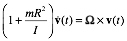 analogous to:
 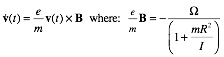 (2.8.31)
A solid ball with inertia I=2/5mR2 leads to an effective cyclotron frequency of 2W/7, that is, the ball will orbit exactly twice for each seven rotations of the table. The actual surface velocity V=W¥r of the table is analogous to a vector potential A=1/2B¥r of a uniform magnetic field as sketched in Fig. 2.8.1. A ping-pong ball has a noticeably higher “charge-to-mass” ratio and cyclotron frequency. To get a lower value one might construct a light plastic ball with a dense core of tungsten or uranium.
Appendix 2.A. Complex analysis of charge-mass trajectory in uniform crossed E and B fields
Complex variables give concise equations for mass-m of charge-e in electric E and magnetic B fields.
 or:
or: 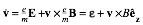 (2.A.1a)
Shorthand notation is used. 

 (2.A.1b)
We let the usual Gibb’s vector notation be restricted to 2D(x,y) motion normal to B-field z-direction.
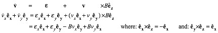 (2.A.2)
This suggests more concise complex variables for velocity and electric field
 .
.
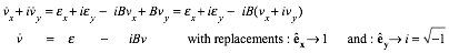 (2.A.3)
A velocity transformation may cancel the constant ε-field to give an equation
  .
.
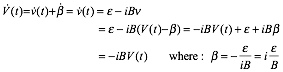 (2.A.4)
An exponential V(t)=e-iBtV(0) solution results. As noted in Unit 1 (10.27), e-iBt is a clockwise 2D rotation.
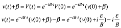 (2.A.5a)
Expanding e-iBt, , and
, and  reveals x (Real) and y (Imaginary) components seen in (2.8.21).
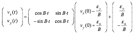 (2.A.5b)
Integrating (2.A.5a) yields complex coordinate q=x+iy affected by both ex and ey. (Compare to (2.8.22).)
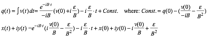 (2.A.6a)
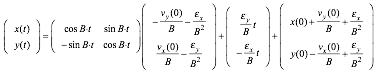 (2.A.6b)
For positive magnetic  the mass m moves as though attached to a clockwise rotating disc that also translates perpendicular to the applied E-field. The path follows a generalized cycloid that is curlate for relatively slow translation and prolate for faster translation. A normal cycloid results for zero initial velocity. This case is given first below and compared to paths of points on a hammered flying stick.
A +y-field electric (ex=0 and ey>0) and zero initial values (q(0)=0=v(0)) gives a horizontal cycloid traced by a circle of radius R=εy/B2 rolling through angle θ=B·t and horizontal x-distance R·θ=B =ey·t/B.
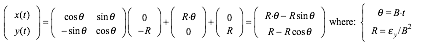 (2.A.7)
If you hammer a stick at a point h meters from its center you give it some linear momentum P and angular momentum L = h·P as shown in Fig. 2.A.1 below. The resulting angular velocity w about the center is the angular momentum L divided by the moment of inertia I= M l2/3 of the stick.
w = L / I (= 3 L /(M l2) for stick) (2.A.8a)
= h P / I (= 3 hP /(M l2) for stick) (2.A.8b)
This depends on the hitting radius h and is zero when h=0. Otherwise, points on the stick follow cycloids that are variously curlate or prolate. One point P, called center of percussion (CoP), is on a normal cycloid made by a circle of radius p rolling on an imaginary road thru P in direction of P. This is the point on the wheel where speed pw due to rotation just cancels the translational speed of the stick center.
P /M =VCenter =|pw|= 3 p·hP /(M l2) (2.A.9)
Solving gives the percussion radius p of the CoP point that has no velocity just after the hammer hits at h.
p = l2/3h (2.A.10)
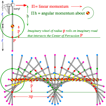
Fig. 2.A.1 Cycloidic paths due to hitting a stationary stick.
Exercise 2.8.1The cycloidal path solutions (2.8.23) include a straight-line path. Describe initial conditions that give a line path.
Exercise 2.8.2How might the mechanical analog of cyclotron orbits change the charge-to-mass ratio (e/m), that is, the ratio of orbit-to-table revolutions? What experimental range is available?
Writing theory and equations is one thing and understanding what it all means is quite another. Application of theory is certainly satisfying if not the most satisfying part of mechanics or, perhaps any branch of physics. Very often it only there that you finally get the theory right!
This section includes a discussion of the trebuchet and its relation to human dynamics or kinesiology and mechanics of lever-sports like tennis or golf. So if you like doing one of these sports or you just want to impress your significant other by ringing the bell at the fair, then listen up!
A difficult part of learning physics is disabusing an Aristotelian misconception that applied force gives immediate and proportional velocity. It is also a difficult misconception to overcome in lever-sports like tennis, golf, or baseball. Simulations of a trebuchet (Fig. 2.9.1a-b) help show how expert tennis players (Fig. 2.9.1c) can hit precise 70 mph tennis drives but "hackers" can barely control half that speed.
The trebuchet simulation shows how and when energy is transferred from the big mass M to the much smaller projectile m. The only power channel to mass m is the tension vector F along the rope l. Since power is the scalar product F•v of force and velocity v, the big lever rb has to do all its work early on when F and v are nearly collinear and well before the rope swings out perpendicular to velocity v. (Then F•v becomes zero or negative.) The later trajectory in Fig. Fig. 2.9.1 b serves only to steer mass m.
The trick is to get energy into m at the lever end (racquet head) early when it is well behind the point where the energy is going to be used. An early force F is more effective pulling along lever arm-l (analogous to a nearly rigid arm-and-racquet handle) as the mass m (racquet head) begins to swing out due to centrifugal force as in Fig. 2.9.1a. Furthermore, a large force is produced early and automatically by the massive trebuchet (or player body) pulling along the l-lever as the body M rotates. Seemingly effortless tennis power comes from the stronger leg and abdominal flexors rotating one's body analogously to gravity rotating the trebuchet main beam and not from pectoral or arm muscles (of which the trebuchet has none at all.) The shoulder joint should be a relaxed and loose hinge, not a hacking power source.
A common tennis or golf coach's mantra is, "Rotate your body!" but few will (or can) explain the Galilean relativity behind the mantra. Perhaps, the analogy with the trebuchet can help clarify this. Like the trebuchet, expert tennis strokes use the later "follow-through" period to accurately guide and aim a more-or-less rigid arm-racquet system analogous to the trebuchet mass m and lever l. In Fig. 2.9.1c shoulder radius is rb and l is the radius from shoulder to CM of arm-racquet. (l is radius of gyration.) In the follow-through phase, the arm-racquet system, like the trebuchet mass m, has already gained its energy easily and early by rb rotation pulling along a nearly rigid l. So, the remaining time before ball contact may be devoted to relatively small corrections of flight of l without needing late and ineffectual "hacking" acceleration. Simply put, the shoulder lever or beam rb provides a moving body frame that smoothly "throws" the arm-racquet system-l at the ball.
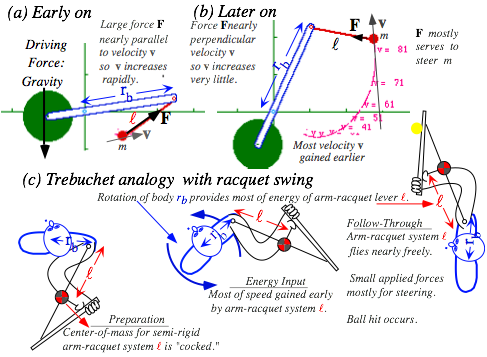
Fig. 2.9.1 Example of elementary trebuchet dynamics and qualitative analogy with tennis racquet swing
Another coach's mantra is, "Let the racquet (or driver) do the work!" Arm muscles should be practically rigid so as to do little work that helps or hinders the flight. Relatively loose shoulder muscles are like a trebuchet hinge between beam rb and lever l and should not to hinder (or help) l-speed, either.
In contrast, a "hacker" waits until the racquet head is near the delivery point (Fig. 2.9.1b) and has to apply a large torque, that is, a large perpendicular force-couple to a lower part of lever l. At this late time a long racquet and arm-lever length l acts to one's disadvantage. Poor leverage reduces the acceleration at the delivery end. (Acceleration of outer end of l is inversely proportional to l.) Also, the racquet-arm system, in a desperate attempt to quickly add energy, degenerates into a floppy multi-angle and multi-torque system that has small leverage and is difficult to accurately control. Between the shoulder and the racquet there are (at least) four independent angles in wrist and elbow that correspond to an eight-dimensional phase space. This is a human control-system nightmare and provides a veritable gold-mine for orthopedic surgeons.
It may help to study an anti-analogy to a trebuchet and a well-evolved tennis or golf swing. Before apes and man could throw (or play golf) there were plenty of animals (and microbes) that could swim with simple flagella, flippers, or flinging motions. So for a moment, let’s un-evolve back to our roots!
Consider now a device we will call the "flinger" which seems to (but really doesn't) track one's innate Aristotelian misconceptions about force and velocity. This device is an exact opposite of trebuchet in that it applies most of its force later rather than early and perpendicular rather than along a lever. To use sports analogy, this is like comparing a pass (flinger launch) to a slapshot (trebuchet launch) in hockey.
One common way to make a flinger is to insert a pool queue-stick into a lubricated skateboard wheel which may slide down the tapered stick about a half way before being stopped by the thicker handle. Then the pool stick is cast like a fly-fishing rod so that the wheel flies off with enough speed to go quite a distance. (See Fig. 2.9.4b in the following section.)
Many of us have, at one time or another, done something like this with an apple pierced by a stick. However, apples tend to stick to a stick more than the skateboard wheel does, and so the apple may also get an appreciable initial longitudinal force just like the trebuchet projectile. The wheel on the flinger, however, slides with negligible friction so it cannot take much advantage of trebuchet-like energy transfer. Rather flinging relies solely on orthogonal forces and torques that increase as the stick rotates; its physics is quite the opposite to that of the trebuchet. Also, flinging applies force later rather than earlier and may require large (arm wrenching) torque if the apple is a large one.
A flinger simulation in Fig. 2.9.2 is set up like the trebuchet to be gravity-driven. The projectile energies achieved by the flinger are well below those of the trebuchet with similar mass and lever ratios. However, flinger proponents may object that such a gravity driven device unfairly penalizes flinging which, unlike trebuchet, puts off most of its work until the last moment when its beam is slowing down.
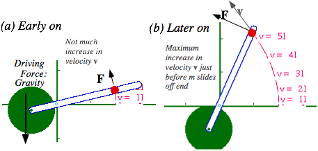
Fig. 2.9.2 Example of elementary "flinger" dynamics and qualitative analysis
To address these objections, let us imagine that either system is mounted on a main beam that turns with constant angular velocity ω as sketched in Fig. 2.9.3. Also, we will handicap the trebuchet by starting it out in a poorer half-cocked initial position as seen in Fig. 2.9.3a. This starting position is more like a 6-o'clock racquet-back-and-ready position often recommended for tennis. (Initially, the racquet handle butt points at the incoming ball and is drawn like a sword toward it.) Full-cocked 8-9 o'clock positions like Fig. 2.9.3b were used by ancient warriors for maximum trebuchet range and are more appropriate for golf or baseball. These are calculated below, too.
For a mass fixed in a rotating frame at radius r the radial outward centrifugal acceleration is ω2r. If the mass is moving with velocity v there is an additional Coriolis acceleration of wxv, but since that is normal to the frictionless constraints of this problem, it can be ignored. Then the rotating frame speed can be calculated using an inverted quadratic effective potential, an “anti-oscillator” if you will.
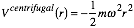 (2.9.1)
The potential is such that its gradient is the centrifugal force.
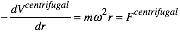 (2.9.2)
It might seem at first that the flinger should win this comparison since radius r(t) for m will grow as a hyperbolic coshω t function that is soon an exponential, while the trebuchet seems limited by its pendulum design. However, we will see the trebuchet is gaining speed at a similar rate, albeit from a starting radius R1 at the 6-o'clock position which has less potential, but the trebuchet finally redirects its mass toward the tangential direction so its velocity adds directly to the rotation in the inertial lab frame while the flinger only flings m along the rotating beam radius.
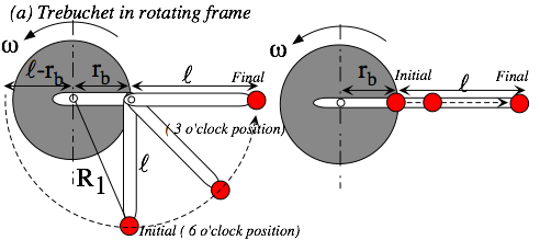
Fig. 2.9.3 Comparing rotating frame dynamics of (a) trebuchet and (b) flinger for similar dimensions
Final beam-relative speed vbeam rel. is found using KE resulting from a difference of potentials (2.9.1) at final radius rf and initial radius r0. (Initial beam-relative velocity is assumed zero and gravity is ignored.)
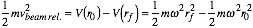 (2.9.3)
The flinger initial radius is r0 = rb and the final radius is rf = rb + l.
 (2.9.4)
The trebuchet final radius is the same but initial radius is: r0 =R1 where: R12 = rb2 +l2 in Fig. 2.9.3a
 (2.9.5)
The inertial lab-relative final velocity for the flinger is a vector sum of the radial velocity  from (2.9.4) and the tangential velocity ω(rb + l ) due to the beam-frame rotation at the end point rf = rb + l.
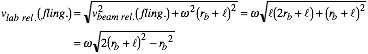 (2.9.6)
The inertial lab-relative final velocity for the trebuchet is a simple sum of the tangential velocity  from (2.9.5) and the tangential velocity ω(rb + l) due to beam-frame rotation at end point rf = rb + l.
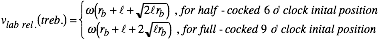 (2.9.7)
The second answer given above is for a fully cocked (9 o'clock) trebuchet It gains by having twice the effective potential drop of a half-cocked (6 o'clock) trebuchet, assuming final release at 3 o'clock.
Here are numerical comparisons, first with rb=2 and l=1 (long beam and short lever)
 (2.9.8a)
then with rb=1.5 and l=1.5 (medium lever and medium beam)
 (2.9.8b)
and finally, with rb=1 and l=2 (short beam and long lever)
 (2.9.8c)
The flinger starts to catch up with the trebuchet as the lever gets longer, but in the examples above, even a half-cocked trebuchet is clearly superior and is delivering 50% to nearly 100% more energy than a flinger.
Also, it should be noted that this ultra-simplified example of a trebuchet favors equal beam and lever lengths (rb=l), something that is generally borne out in more comprehensive numerical simulations. The flinger, on the other hand just wants a longer lever l that would entail excessive torque to keep the flinger moving even for a small projectile mass m. Some ancient trebuchets threw a four or five ton projectile. It is doubtful that anything could fling such a thing!
The approximate trebuchet analysis, ending with equations (2.9.7), also provide estimates for biomechanical energy transfer, specifically ancient pick-axing or wood-chopping, later rail spike driving or ringing the bell at the fair. As noted before in the tennis analogy, the secret is to pull as much as possible along the handle using an abdominal powered rotating torso. Shoulder muscle contraction helps, too, but generally should not be wasted applying forces transverse to the lever. Assuming the optimal ratio of torso length rb and lever l (rb=r=l), the expected final velocity (2.9.7) for the hammer head m should be approximately 4rω with energy 8mr2ω2. For a torso and lever length of r=2.5 feet and an average torso rotation rate of ω=5 radians/second gives a velocity of 50 feet/s. For an 8lb (or 1/4 slug) hammer head, the kinetic energy is 500 ft.lbs. that (disregarding friction) sends a 10lb ringer up to 50 ft. (Ringers are usually less than 5lbs, so this is a fairly conservative estimate.)
Short of pick-axing or fair-bell-ringing, one may compete for distance using either a stick and string arrangement that resembles trebuchet mechanics (Fig. 2.9.4a) or a flinger arrangement (Fig. 2.9.4b). Casting a 1 meter fling stick with a slider m starting at 50 centimeters as shown in Fig. 2.9.4b provides an easy comparison to casting a 50 centimeter stick and hook holding a 50 centimeter string-pendulum made from the same mass m (a skateboard wheel) as sketched in Fig. 2.9.4a. Fig. 2.9.4 is a rough attempt at the comparison in Fig. 2.9.3.
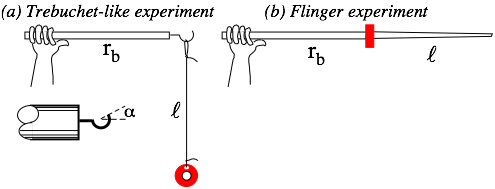
Fig. 2.9.4 Simple experiments for comparing dynamics of (a) trebuchet (b) flinger for similar dimensions.
While good for hours of fun, these experiments can easily degenerate into some pretty sorry science. There are several reasons for this, all interesting in themselves. Most penalize the trebuchet model.
First, what is about to happen in Fig. 2.9.4 may not correspond to Fig. 2.9.3. One tends to throw the flinger rather than just rotating it. Due to unavoidable longitudinal "stiction" the flinger can gain some of the longitudinal advantage of trebuchet-like acceleration. In any case, it is hard to make sticks rotate with constant angular velocity unless attached to a machine. An initial jerk is necessary to start a launch.
Second, humans are natural flingers (like most animals going back to primitive fish). Throwing or any sort of trebuchet-like dynamics requires skill and coaching to be optimal. One is likely to be more comfortable, at first, with the (Aristotelian) flinger unless one does fly-casting or some related activity.
Third, the curve and angle a of the release hook on the trebuchet-model stick is critical. Usually, a=0 gives the optimal range but small variations may be desired for different throwing styles. Release settings are the bane of trebuchets. Failure of Cortez's ingeniators to set the proper release angle is rumored to have resulted in the projectile going straight up and destroying the machine on its first shot! [1] With the device in Fig. 2.9.4a, it is quite easy to shoot yourself in the foot or more sensitive body parts. Cuidado!
There is another universal modern human activity called twiddling: swinging one's glasses, keys or a key ring during periods of contemplation or procrastination. Such motion is related to that of the trebuchet and to some other phenomena such as quantum waves that might have seemed, at first, totally unrelated.
Suppose you are holding a small mass by a string attached to it as sketched in Fig. 2.9.5. This is similar to the trebuchet-model in Fig. 2.9.4a if length l could be assumed large compared to the motions. Wiggling the supporting end of the string may rapidly excite the hanging mass. How rapidly depends on frequency and direction, horizontal x or vertical y, of the wiggle. Horizontal wiggle would be the most natural for most and leads to ordinary (linear) resonance. However, as shown below, vertical wiggle may cause much more rapid excitation if done correctly and corresponds to parametric or nonlinear resonance which is described (for small angles) by an equation similar to the Schrodinger wave equation. [6]
The equations of motion can be derived quite easily by applying the equivalence principle to the accelerating frame attached to the pendulum support or hook at the end of a trebuchet beam. According to this, it is only necessary to subtract the acceleration vector a of an oscillating frame from the usual vertical gravity acceleration vector g to obtain the effective gravity  experienced by the pendulum.
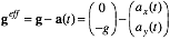 (2.9.9)
If the support is oscillating in the horizontal direction according to X0(t)=Axcos(ωx t+ax) and in the vertical direction according to Y0(t)=Aycos(ωy t+ay), then the acceleration vector is
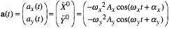 , (2.9.10)
for arbitrary constant amplitudes Ax, Ay, and phases ax, and ay. This gives the effective gravity vector.
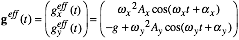 (2.9.11)
The general jerked-pendulum equation of motion in such a  field is the following.
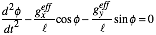 (2.9.12)
For small angles (cos φ~1 and sin f~φ ) this reduces to
 . (2.9.12a)
Two cases indicated in Fig. 2.9.5 are X-force: Ax>0, Ay=0 with phase ax = a for linear resonance
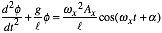 , (2.9.12b)
or Y-force parametric resonance: Ax=0, Ay>0 with ay = p so Y(t) accelerates upward from at t=0.
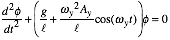 (2.9.12c)
The latter is like a Schrodinger wave equation. (With a cosine potential it is a Mathieu equation.[6])
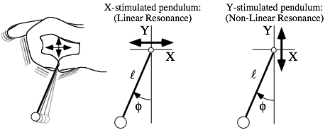
Fig. 2.9.5 Two (very different) types of accelerated pendulum resonance.
Most physicists know of these equations as functions of spatial dimension x.
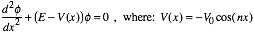 (2.9.12d)
Here time t replaces coordinate x as the independent variable, and y-effective gravity -ay(t)/l replaces potential V(x). This equation is known for having Gaussian super-exponential  (or in our case
 ) asymptotic solutions. So the trebuchet is capable of even faster acceleration than the flinger’s impressive exponential growth. It is also more likely to undergo chaotic behavior.
The linear harmonic resonance turns out to grow only linearly, but it is the most common resonance mechanism in terms of the mechanics of our human visual, audio, and vocal systems Both these examples of resonance have detailed treatments in the Unit 4 devoted to waves and resonance. There we will take up the more complicated and powerful parametric resonance.
What about a trebuchet in space? Galileo’s generals would certainly laugh that idea out of the Vatican! But if a rocket blast could impart beam momentum, then throwing ability would be recovered. And, this time the Hamiltonian problem has analytic solutions. The trebuchet Hamiltonian for zero gravitational potential (g=0=V) is a function only of the beam-relative angle φB = φ - q - p/2. A coordinate transformation based on Fig. 8 takes advantage of this.
φB = φ - q - p/2 (2.9.13a) φ = φB + θB + p (2.9.13c) θB = θ + p/2 (2.9.13b) θ = θB - p/2 (2.9.13d)
The velocities (for a Lagrangians) and momenta (for our Hamiltonian) are transformed by Jacobians.
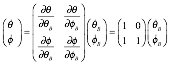 (2.9.14a)
 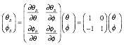 (2.9.14b)
Transformation of momenta pk is transpose-inverse to that of  so Poincare's invariant (2.6.9) is!
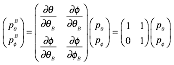 (2.9.15a)
 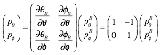 (2.9.15b)
(p•v must be invariant to coordinate transformation.) The transformed Hamiltonian is found by writing qk in terms of qmB using (2.9.13c-d) and pk in terms of pmB using (2.9.15b) and substituting into (2.6.9d).
(2.9.16)
 When gravity is zero, the qB-angular momentum is constant (pqB = L=const.) according to (2.6.16). This combined with energy conservation (2.6.15) gives the following for the (g=0) case.
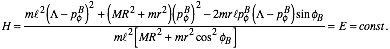 (2.9.17)
This is a quadratic equation relating φB-angular momentum pfB to angle φB and constants L and E.
 (2.9.18a)
 (2.9.18b)
The total effective moment of inertia I of the main beam (if m were stuck on the hook end) is defined by
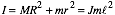 . (2.9.18c)
If one is seeking kinetic quantities, that is, final velocities, it helps to rewrite conserved momenta pqB = L and energy H=E=T (for g=0) in terms of desired angular velocities ( ) using (2.4.2) and (2.9.15a).
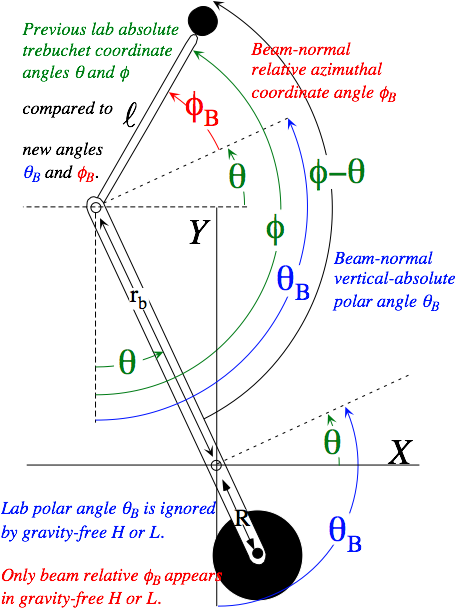
Fig. 2.9.6 Lab (q,f) and beam-normal (θB,fB) relative coordinates for trebuchet. (Each value is positive.)
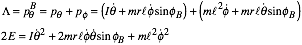 (2.9.19a)
For sake of simplicity, we consider the trebuchet for which beam and rope are equal length (r=l).
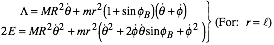 (2.9.19b)
(2.9.19) is found for three relative positions 9 o'clock (fB=-π/2), 6 o'clock (fB=0), and 3 o'clock (fB=π/2) shown by Fig. 2.9.7a-c. Since total angular momentum L and energy E remain constant at all three positions, that is, independent of φB and θB, the differing velocities ( ), (
), ( ), or (
 ) at the different positions are easily related to each other.
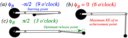
Fig. 2.9.7 Extreme beam-relative coordinate positions for trebuchet throwing sequence.
If the rope or lever-l is tucked in along the main beam at 9 o'clock then φB=-π/2 so (2.9.19b) reduces to
 (2.9.20a)
We will assume φB=-π/2 is the initial position where both angles have the same initial velocity ω. If the rope or lever-l is normal to the main beam (at 6 o'clock in Fig. 2.9.7b) then φB=0 so (2.9.19b) reduces.
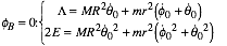 (2.9.20b)
If the rope or lever-l is stretched out along the main beam at 3 o'clock then φB=π/2 so (2.9.19b) reduces.
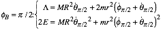 (2.9.20c)
We take 9 o'clock (φB=π/2) to be a launch position that, presumably, would provide the greatest velocity for the projectile m. According to (2.2.13) and (2.3.9) mass m has the following KE and speed v.
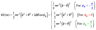 (2.9.21a)
Final projectile speed is
 . (2.9.21b)
Equating final (L,E) in (2.9.20c) to initial (L,E) in (2.9.20a) gives easily solved equations.
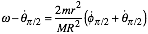 (2.9.22a)
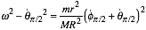 (2.9.22b)
Dividing (2.9.22b) by (2.9.22a) gives a linear relation.
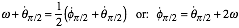 (2.9.22c)
If the main beam is massive compared to the projectile (M>>m), then its angular velocity may remain fairly constant, so its initial velocity  is not significantly greater than the final velocity
  . Then by (2.9.22c) the projectile lever or rope l has final angular velocity 3 times that of the beam:
  .
.
Substituting this approximation into the KE and speed formula (2.9.21) for φB=π/2 gives a kinetic energy that is sixteen times that of a mass on the end of the r-beam where m rides on a simple catapult.
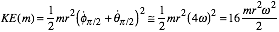 (2.9.23a)
This amounts to a projectile velocity (2.9.21b) that approaches four times the speed of the beam tip.
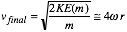 (2.9.23b)
This is consistent with the result v= in (2.9.7) for a constant-ω model with rb=l in the case for which it starts full-cocked in a 9 o'clock initial position and releases at 3 o'clock.
However, this model tells what angular velocity the beam loses. Substituting  from (2.9.22c) into (2.9.22a) shows that the final beam angular velocity
  can be reduced to zero or negative values.
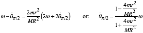 (2.9.24)
The case MR2=4mr2 is interesting because the beam is stopped completely while giving 100% of its energy to the projectile. With  the projectile angular velocity ends up 2 times that of the initial beam angular velocity (
 according to (2.9.22c)) instead of 3 times which is the limit for small m.
These results are reminiscent of those for a super-ball-pen or tower described in Unit 1 and in ref. [7]. In those experiments, a superball of mass M descends to the floor with a smaller object m riding on top. If the rider is of negligible mass m compared to M, it is bounces skyward at three times the initial contact velocity. (Recall Fig. 1.2.5) But if mass m is just large enough (that is m=M/3) to stop M and take all its energy, then it is thrown skyward at just twice the initial velocity.
Relating the simple gravity-free kinetic theory above to a gravity driven trebuchet is problematic, to say the least. One is left to devise a number of estimation schemes. For example, the initial beam angular velocity w could be derived from the average velocity  of a gravity driven beam with projectile m fixed at some average position, say at the 6 o'clock position. For m/M<<1 this can be (over)estimated to be the average angular velocity of a pendulum of length R falling angle π/2 from the 9 o'clock initial position in Galileo's approximation.
 (2.9.25)
The reproductions of 13th-century trebuchets in Ref. [2] were based on drawings from ingeniums used in the 1215 Siege of Kenilworth. The modern-day ingeniators used twelve to thirteen thousand pounds of lead and sand to throw a 250 pound stone ball, that is, M/m~50. Had they used the criterion MR2=4mr2 for 100%-energy transfer from (2.9.24) their trebuchet would have a ratio r/R = √50/2=3.5 of the throwing beam to driving beam radii. Instead, the drawings show that l~r~42 ft. is about 3.7 times the driving radius R of the sand box M. Using (2.9.22) to (2.9.25) with 100% energy transfer assumption we find the following approximate launch velocity.
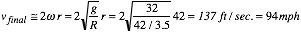 (2.9.26)
As one might expect, this 100% estimate is below the 100 to 120 mph. velocities achieved in Ref. [2]. By assuming the correct ratio of radii in using (2.9.22) to (2.9.25), one can bring the estimate closer.
Accurate theoretical simulation or prediction of trebuchet launches such as those described in Ref. [2] generally requires analytical and numerical techniques such as those described in Sec. 2.10. For one thing, Ref. [2] described a trebuchet with wheels that moved forward and thereby added translation velocity to the projectile. This involves a translation degree of freedom x and carriage mass μ as shown in Fig. 2.9.8. Each degree of freedom makes analytical solutions more difficult and numerical simulation more necessary.
As long as numerical techniques are used, one may as well improve the stick-and-ball pendulum models so they account for the compound pendulums whose radii of gyration are generally smaller than the geometric radii. The discrepancy between inertial and geometric radii is most obvious in discussions of the analogy with tennis racquet dynamics involving Fig. 2.9.1c, but most trebuchets could use this correction, as well.
Last but not least, most trebuchets have their big mass M hanging as a pendulum, too, just like the little mass m that is the projectile. This lends at least one more degree of freedom. So sorry, Galileo! This is one tough problem.
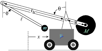
Fig. 2.9.8 Trebuchet with translation uncoil and recoil allowed.
Modern materials and analysis also open the possibility of serial-segment trebuchets such as the triple segmented device sketched in a simulation shown by Fig. 2.9.9. A trebuchet with more than two moving parts is easily capable of exceeding the upper limit of  and vfinal=4ωr that limits two-part machines. In Sec. 1.8 of Unit 1 it was shown how superball towers with n=3, 4, 5,... parts can, in principle, achieve very high velocity.
A multi-segment trebuchet is analogous to a baseball pitch and a tennis serve, the latter of which is achieving extraordinary velocities in world-class play. More simply, the multi-segment trebuchet is like a (sometimes dangerous) "crack-the-whip" game played by a chain of children on skates. More to the point, such a device could be modeled after a bullwhip.
One wonders, "Could a gravity driven multi-trebuchet actually throw a massive object faster than the speed of sound?" Certainly a spring, motor or hand driven device can exceed 700 mph. For centuries it was done daily using bullwhips on Southern and Latin American cattle ranches. (It is said that semi-tropical cowhands were called "Crackers" for this reason.) But, getting such kinetic energy solely from a large mass potential Mgh would require some extraordinary physics and engineering. The PE of M=50 kg mass raised 1 m equals the KE of a m=1 gm mass traveling v=1km/sec. or 2,215 mph or about Mach 3, according to a simple energy equation.
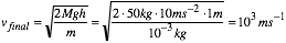 . (2.9.27)
This is reduced to Mach 1 for a 1 gm mass powered by a 5.5 kg mass or a 0.18 gm mass powered by a 1kg weight. The latter begins to sound practical, but it assumes that 100% transfer is possible for each trebuchet segment. However, it remains to be seen if the 2-segment analysis leading to (2.9.22) through (2.9.24) may be applicable to a multi-segmented device.
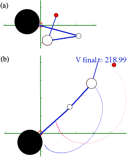
Fig. 2.9.9 Non-optimized example of simulated 3-stage trebuchet dynamics.
(a) Inital position state. (b) Just after launch.
Instead, a better model for a multi-segment device may be that of a bull-whip wave traveling from the heavier end toward the lighter segments and gradually increasing velocity at each joint. Again, this is very similar to the dynamics of the superball tower analyzed in Ref. [7]. Under the right conditions the independent 2-particle collision model was applicable to N-superball amplification. Such multi-stage dynamics have a relativistic version in stellar models of super-novae and the resulting kinetic transfer is called super-elastic-bounce.[8]
Such a complex and high speed system is likely to require numerical simulation to accompany its construction and engineering. Optimal control theory techniques (See Unit 7) should help find the best designs and initial settings. A student using a computer can try more different settings in five minutes than all the ingeniators of the world did in five centuries! High speed digital video tracking of real lab devices can be used to calibrate and check the numerical simulations each time another segment is added to the device. Bending of segments may also be important as it certainly was for the great thirty-ton wooden trebuchets of the 11-th century.
Each increase in speed will bring even larger increases in frictional loss of energy. Friction can only be modeled semi-emperically so the video input coupled with numerical computer graphical techniques will become more essential as the device gains complexity. (Perhaps the whole experiment could be done in a vacuum, but what fun would it be, if you can't hear the "Crack!")
1. Paul E. Chevedden, Les Eigenbrod, Vernard Foley, and Werner Soedel, "The Trebuchet",
Scientific American 273, 66-71 (July 1995).
2. Evan Hadingham and Patrick Ward, "Ready, Aim, Fire!", Smithsonian (January 2000) p. 80.
3. Ref. 1 p.69.
4. Literature search beyond the above references reveals a number of exercises in computer synthesis of the trebuchet, but practically no physical analysis. It is this imbalance that we seek to begin correcting. The ingenium was invented by engineers. (Or, they were invented by it.) Physicists seem quite late coming to this party.
5. William G. Harter, Quantum Theory for the Computer Age (U of A Course 5301 Text (Unpublished)).
6. Jon Mathews and R. L. Walker, Mathematical Methods for Physics (Benjamin, NewYork, 1964) p. 189; The mechanical analogy is discussed extensively in Ref.5 .
ich ss of W. G. Harterif you c7. Class of W. G. Harter, "Velocity Amplification in Collision Experiments Involving Superballs,"
Am. J. Phys. 39, 656 (1971) (A class project which received NBC news coverage).
8. S. E. Wollsley, and M. M. Phillips, "Super-Nova 1987A!" Science 240, 750 (May 1988).
Unit 1.1 Problems
Exercise
3.1.1